Dense neural network with PyTorch

2.2. Dense neural network with PyTorch#

Authors: Javier Duarte, Tyler Mitchell, Raghav Kansal

Run this cell to download the data if you did not already download it in from Tutorial #1:

!mkdir -p data
!wget -O data/ntuple_4mu_bkg.root https://zenodo.org/record/3901869/files/ntuple_4mu_bkg.root?download=1
!wget -O data/ntuple_4mu_VV.root https://zenodo.org/record/3901869/files/ntuple_4mu_VV.root?download=1

import torch
import numpy as np
import pandas as pd
import uproot

2.2.1. Loading `pandas` DataFrames#

Now we load two different NumPy arrays. One corresponding to the VV signal and one corresponding to the background.

# Copy TTree HZZ4LeptonsAnalysisReduced into a pandas DataFrame
treename = "HZZ4LeptonsAnalysisReduced"
filename = {}
upfile = {}
df = {}

filename["VV"] = "data/ntuple_4mu_VV.root"
filename["bkg"] = "data/ntuple_4mu_bkg.root"

# Drop all variables except for those we want to use when training.
VARS = ["f_mass4l", "f_massjj"]

upfile["VV"] = uproot.open(filename["VV"])
upfile["bkg"] = uproot.open(filename["bkg"])

df["bkg"] = upfile["bkg"][treename].arrays(VARS, library="pd")
df["VV"] = upfile["VV"][treename].arrays(VARS, library="pd")

# Make sure the inputs are well behaved.
df["VV"] = df["VV"][(df["VV"][VARS[0]] > -999) & (df["VV"][VARS[1]] > -999)]
df["bkg"] = df["bkg"][(df["bkg"][VARS[0]] > -999) & (df["bkg"][VARS[1]] > -999)]

# add isSignal variable
df["VV"]["isSignal"] = np.ones(len(df["VV"]))
df["bkg"]["isSignal"] = np.zeros(len(df["bkg"]))

2.2.2. Dividing the data into testing and training dataset#

We will split the data into two parts (one for training+validation and one for testing). We will also apply “standard scaling” preprocessing: http://scikit-learn.org/stable/modules/generated/sklearn.preprocessing.StandardScaler.html i.e. making the mean = 0 and the RMS = 1 for all input variables (based only on the training/validation dataset).

# Combine signal and background into one DataFrame then split into input variables and labels.
NDIM = len(VARS)
df_all = pd.concat([df["VV"], df["bkg"]])
dataset = df_all.values
X = dataset[:, 0:NDIM]
Y = dataset[:, NDIM]

# Split into training and testing data.
from sklearn.model_selection import train_test_split

X_train_val, X_test, Y_train_val, Y_test = train_test_split(X, Y, test_size=0.2, random_state=7)
print(X_train_val)
print(X)

# preprocessing: standard scalar (reshape inputs to mean=0, variance=1)
from sklearn.preprocessing import StandardScaler

scaler = StandardScaler().fit(X_train_val)
X_train_val = scaler.transform(X_train_val)
X_test = scaler.transform(X_test)

# Split again, this time into training and validation data.
X_train, X_val, Y_train, Y_val = train_test_split(
    X_train_val, Y_train_val, test_size=0.2, random_state=7
)

[[ 123.59499359 1071.21447754]
 [ 124.97003174 1074.65454102]
 [ 124.32479095  643.70874023]
 ...
 [  87.93131256  538.8001709 ]
 [ 120.99951935  772.50964355]
 [  90.16904449  194.7850647 ]]
[[ 125.07710266 1300.42687988]
 [ 124.2381134   437.22186279]
 [ 124.48066711 1021.74407959]
 ...
 [  89.28808594   53.66157913]
 [ 146.75657654   71.16202545]
 [ 218.86941528   98.91469574]]

2.2.3. Define the model#

We’ll start with a dense (fully-connected) NN layer. Our model will have a single fully-connected hidden layer with the same number of neurons as input variables. The weights are initialized using a small Gaussian random number. We will switch between linear and tanh activation functions for the hidden layer. The output layer contains a single neuron in order to make predictions. It uses the sigmoid activation function in order to produce a probability output in the range of 0 to 1.

We are using the binary_crossentropy loss function during training, a standard loss function for binary classification problems. We will optimize the model with the Adam algorithm for stochastic gradient descent and we will collect accuracy metrics while the model is trained.

# Build our model.
import torch

model = torch.nn.Sequential(torch.nn.Linear(2, 1), torch.nn.Sigmoid())

# Use Binary Cross Entropy as our loss function.
loss_fn = torch.nn.BCELoss()

# Optimize the model parameters using the Adam optimizer.
learning_rate = 0.001
optimizer = torch.optim.Adam(model.parameters(), lr=learning_rate)

# Get validation data ready
val_data = torch.from_numpy(X_val).float()
val_label = torch.from_numpy(Y_val).float()

2.2.4. Run training#

Here, we run the training.

from tqdm import tqdm  # for progress bar while training

losses, val_losses = [], []
min_loss, stale_epochs = 100.0, 0

# 500 epochs.
batch_size = 1024
for t in tqdm(range(500)):
    batch_loss, val_batch_loss = [], []

    for b in range(0, X_train.shape[0], batch_size):
        X_batch = X_train[b : b + batch_size]
        Y_batch = Y_train[b : b + batch_size]
        x = torch.from_numpy(X_batch).float()
        y_b = torch.from_numpy(Y_batch).float()
        y_b = y_b.view(-1, 1)

        # Forward pass: make a prediction for each x event in batch b.
        y_pred = model(x)

        # Get the labels.
        label = y_b
        y = label.view_as(y_pred)  # reshape label data to the shape of y_pred

        # Compute and print loss.
        loss = loss_fn(y_pred, y)
        batch_loss.append(loss.item())

        # Before the backward pass, use the optimizer object to zero all of the
        # gradients for the variables it will update (which are the learnable
        # weights of the model). This is because by default, gradients are
        # accumulated in buffers( i.e, not overwritten) whenever .backward()
        # is called. Checkout docs of torch.autograd.backward for more details.
        optimizer.zero_grad()

        # Backward pass: compute gradient of the loss with respect to model
        # parameters
        loss.backward()

        # Calling the step function on an Optimizer makes an update to its
        # parameters
        optimizer.step()

        # Let's look at the validation set.

        # Torch keeps track of each operation performed on a Tensor, so that it can take the gradient later.
        # We don't need to store this information when looking at validation data, so turn it off with
        # torch.no_grad().
        with torch.no_grad():
            # Forward pass on validation set.
            output = model(val_data)

            # Get labels and compute loss again
            val_y = val_label.view_as(output)
            val_loss = loss_fn(output, val_y)
            val_batch_loss.append(val_loss.item())

            # Monitor the loss function to prevent overtraining.
            if stale_epochs > 20:
                break

            if val_loss.item() - min_loss < 0:
                min_loss = val_loss.item()
                stale_epochs = 0
                torch.save(model.state_dict(), "pytorch_model_best.pth")
            else:
                stale_epochs += 1

    losses.append(np.mean(batch_loss))
    val_losses.append(np.mean(val_batch_loss))

100%|███████████████████████████████████████████████████████████████████████████████████████████████████████████████████████████████████████████████████████████████████████████████████████| 500/500 [00:05<00:00, 88.70it/s]

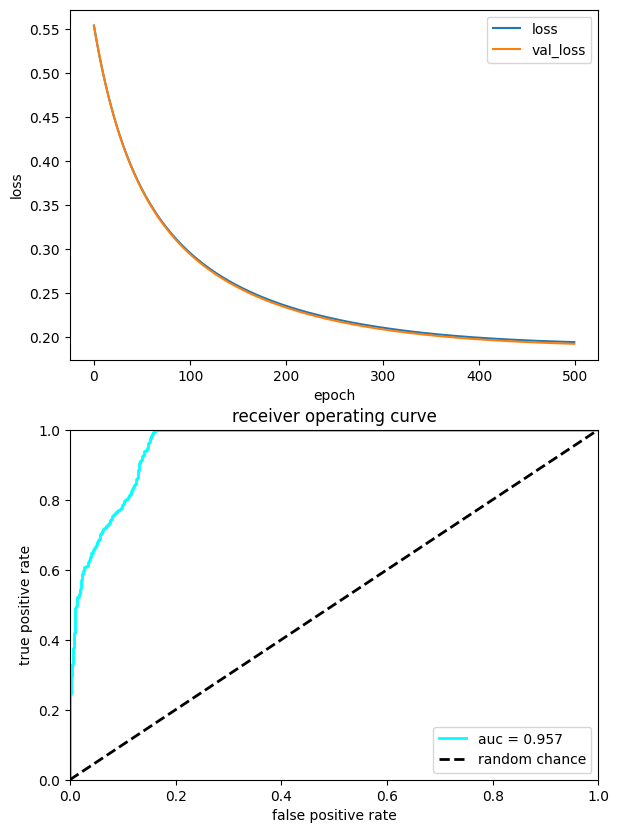
2.2.5. Plot performance#

Here, we plot the history of the training and the performance in a ROC curve

import matplotlib.pyplot as plt

%matplotlib inline

with torch.no_grad():
    # plot loss vs epoch
    plt.figure(figsize=(15, 10))
    ax = plt.subplot(2, 2, 1)
    ax.plot(losses, label="loss")
    ax.plot(val_losses, label="val_loss")
    ax.legend(loc="upper right")
    ax.set_xlabel("epoch")
    ax.set_ylabel("loss")

    # Plot ROC
    X_test_in = torch.from_numpy(X_test).float()
    Y_predict = model(X_test_in)
    from sklearn.metrics import roc_curve, auc

    fpr, tpr, thresholds = roc_curve(Y_test, Y_predict)
    roc_auc = auc(fpr, tpr)
    ax = plt.subplot(2, 2, 3)
    ax.plot(fpr, tpr, lw=2, color="cyan", label="auc = %.3f" % (roc_auc))
    ax.plot([0, 1], [0, 1], linestyle="--", lw=2, color="k", label="random chance")
    ax.set_xlim([0, 1.0])
    ax.set_ylim([0, 1.0])
    ax.set_xlabel("false positive rate")
    ax.set_ylabel("true positive rate")
    ax.set_title("receiver operating curve")
    ax.legend(loc="lower right")
    plt.show()

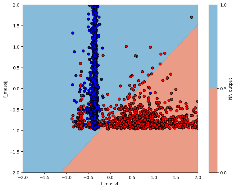
../_images/dc086d8f07429830020318103baf06b701a0b0ee4ba81b040ff8b11aee9f15ca.png

2.2.6. Plot NN output vs input variables#

Here, we will plot the NN output and devision boundary as a function of the input variables.

# make a regular 2D grid for the inputs
myXI, myYI = np.meshgrid(np.linspace(-2, 2, 200), np.linspace(-2, 2, 200))
# print shape
print(myXI.shape)
myZI = model(torch.from_numpy(np.c_[myXI.ravel(), myYI.ravel()]).float())
myZI = myZI.reshape(myXI.shape)

(200, 200)

The code below shoes how to plot the NN output and decision boundary. Does it look optimal?

from matplotlib.colors import ListedColormap

plt.figure(figsize=(20, 7))

# plot contour map of NN output
# overlaid with test data points
ax = plt.subplot(1, 2, 1)
cm = plt.cm.RdBu
cm_bright = ListedColormap(["#FF0000", "#0000FF"])

cont_plot = ax.contourf(myXI, myYI, myZI > 0.5, cmap=cm, alpha=0.8)
ax.scatter(X_test[:, 0], X_test[:, 1], c=Y_test, cmap=cm_bright, edgecolors="k")
ax.set_xlim(-2, 2)
ax.set_ylim(-2, 2)
ax.set_xlabel(VARS[0])
ax.set_ylabel(VARS[1])
plt.colorbar(cont_plot, ax=ax, boundaries=[0, 1], label="NN output")

plt.show()
# plot decision boundary
# overlaid with test data points

../_images/4f5f076f4ce1ff7d6e3196ac847967f7838fc0a2cddedf4c9d6d1cf9a5e90a5f.png

Question 1: What happens if you increase/decrease the number of hidden layers?

Question 2: What happens if you increase/decrease the number of nodes per hidden layer?

Question 3: What happens if you add/remove dropout?

Question 4: What happens if you add/remove early stopping?