3. Convolutional Neural Networks for Jet-Images#
Authors: Javier Duarte, Raghav Kansal
3.1. Introduction#
Introduction adapted from CoDaS-HEP 2023
In this part you will learn how to build and train a Convolutional Neural Network (CNN). For this exercise, we will use the dataset containing jet images and corresponding labels.
Traditional approaches to jet tagging rely on features, such as jet substructure, designed by experts that detect characteristic energy deposit patterns. In recent years, many studies applied computer vision for event reconstruction at particle colliders. This was obtained by projecting the lower level detector measurements of the emanating particles onto a cylindrical detector and then unwrapping the inner surface of the calorimeter on a rectangle. Such information was further interpreted as an image with calorimeter cells as pixels, where pixel intensity maps the energy deposit of the cell, i.e. jet images. The different appearance of these jets can be used as a handle to discriminate between them, i.e. jet tagging.
While you can use transform images to work with dense networks, CNNs are better suited. Instead of transforming the data, we modify the architecture of the network to work with 2D/3D matrices: (from this great page)

As the name suggestions, the main operation inside a CNN is the convolution layer.
3.1.1. Convolution Operation#
Two-dimensional convolutional layer for image height \(H\), width \(W\), number of input channels \(C\), number of output kernels (filters) \(N\), and kernel height \(J\) and width \(K\) is given by:
\begin{align} \label{convLayer} \boldsymbol{Y}[v,u,n] &= \boldsymbol{\beta}[n] + \sum_{c=1}^{C} \sum_{j=1}^{J} \sum_{k=1}^{K} \boldsymbol{X}[v+j,u+k,c], \boldsymbol{W}[j,k,c,n],, \end{align}
where \(Y\) is the output tensor of size \(V \times U \times N\), \(W\) is the weight tensor of size \(J \times K \times C \times N\) and \(\beta\) is the bias vector of length \(N\) .
The example below has \(C=1\) input channel and \(N=1\) (\(J\times K=3\times 3\)) kernel credit:
Some terminology:
kernel: The matrix which is convolved with the image. The parameters of this matrix are what need to be learnt.
stride: The amount by which the kernel is translated for each output (above, it is 1).
padding: How to deal with with the edges of the image (here, we’re using “same” padding)
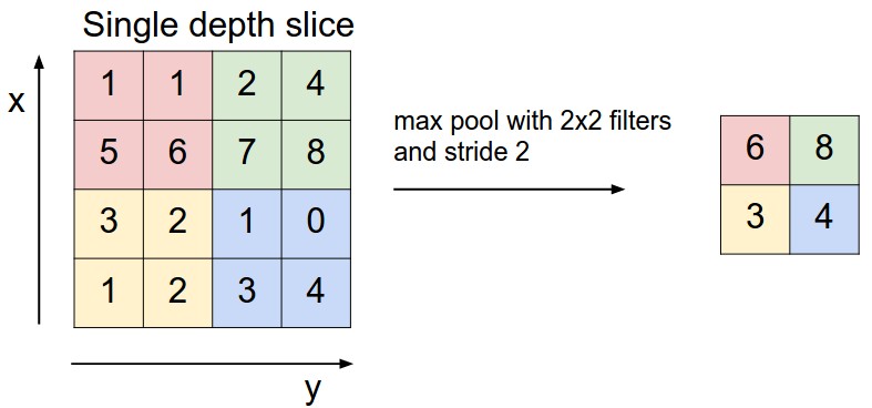
3.1.2. Pooling#
We also add pooling layers to reduce the image size between layers. For example, max pooling: (also from here
3.2. Load numpy arrays#
Now let’s implement a CNN using Keras. Here, we load the numpy arrays containing the 4D tensors of “jet-images” (see arxiv:1511.05190).
!mkdir -p data
!wget -O data/jet_images.h5 "https://zenodo.org/record/3901869/files/jet_images.h5?download=1"
Show code cell output
--2023-08-12 00:16:57--  https://zenodo.org/record/3901869/files/jet_images.h5?download=1
Resolving zenodo.org (zenodo.org)... 188.185.124.72
Connecting to zenodo.org (zenodo.org)|188.185.124.72|:443... connected.
HTTP request sent, awaiting response... 200 OK
Length: 85520350 (82M) [application/octet-stream]
Saving to: ‘data/jet_images.h5’

100%[======================================>] 85,520,350  6.41MB/s   in 25s

2023-08-12 00:17:23 (3.21 MB/s) - ‘data/jet_images.h5’ saved [85520350/85520350]
import h5py

h5f = h5py.File("data/jet_images.h5", "r")

jet_images_dict = {}
jet_images_dict["QCD"] = h5f["QCD"][()]
jet_images_dict["TT"] = h5f["TT"][()]

h5f.close()
# 4D tensor (tensorflow backend)
# 1st dim is jet index
# 2nd dim is eta bin
# 3rd dim is phi bin
# 4th dim is pt value (or rgb values, etc.)
print(jet_images_dict["QCD"].shape)
print(jet_images_dict["TT"].shape)
(3305, 30, 30, 1)
(1722, 30, 30, 1)
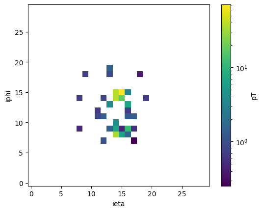
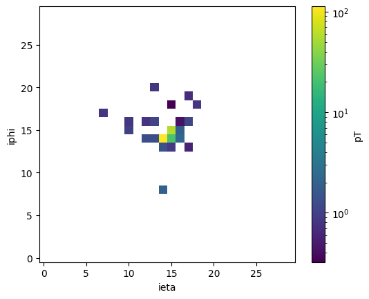
3.3. Plotting jet-images#
Let’s plot some jet-images (individual jets and averaged over all jets)
Question 1: Try to plot the average W and QCD jet-images.
import matplotlib.pyplot as plt
import matplotlib as mpl
import numpy as np

%matplotlib inline

# plot one W jet
i = 7
plt.figure("W")
plt.imshow(
    jet_images_dict["TT"][i, :, :, 0].T,
    norm=mpl.colors.LogNorm(),
    origin="lower",
    interpolation="none",
)
cbar = plt.colorbar()
cbar.set_label("pT")
plt.xlabel("ieta")
plt.ylabel("iphi")
plt.show()

# plot average W jet
# plot one QCD jet
i = 7
plt.figure()
plt.imshow(
    jet_images_dict["QCD"][i, :, :, 0].T,
    norm=mpl.colors.LogNorm(),
    origin="lower",
    interpolation="none",
)
cbar = plt.colorbar()
cbar.set_label("pT")
plt.xlabel("ieta")
plt.ylabel("iphi")
plt.show()

# plot average QCD jet
3.4. Define our convolutional model#
Question 2: Here we have a relatively simple Conv2D model using regularization, batch normalization, max pooling, and a fully connected layer before the ouput. Implement the network defined in https://arxiv.org/pdf/1511.05190.pdf. Compare the performance and number of parameters when using fully connected layers instead of convolutional layers.
import tensorflow.keras.backend as K
from tensorflow.keras.models import Model
from tensorflow.keras.layers import (
    Input,
    Conv2D,
    MaxPool2D,
    Flatten,
    Dropout,
    Dense,
    BatchNormalization,
    Concatenate,
)
from tensorflow.keras.regularizers import l1, l2

nx = 30
ny = 30
inputs = Input(shape=(nx, ny, 1), name="input")
x = Conv2D(
    filters=8,
    kernel_size=(3, 3),
    strides=(1, 1),
    padding="same",
    activation="relu",
    name="conv2d_1",
    kernel_regularizer=l2(0.01),
)(inputs)
x = BatchNormalization(momentum=0.6, name="batchnorm_1")(x)
x = MaxPool2D(pool_size=(2, 2), name="maxpool2d_1")(x)
x = Flatten(name="flatten")(x)
x = Dense(64, activation="relu", name="dense")(x)
outputs = Dense(1, activation="sigmoid", name="output")(x)
model = Model(inputs=inputs, outputs=outputs)
model.compile(optimizer="adam", loss="binary_crossentropy", metrics=["accuracy"])
model.summary()
Model: "model_1"
_________________________________________________________________
 Layer (type)                Output Shape              Param #
=================================================================
 input (InputLayer)          [(None, 30, 30, 1)]       0

 conv2d_1 (Conv2D)           (None, 30, 30, 8)         80

 batchnorm_1 (BatchNormaliz  (None, 30, 30, 8)         32
 ation)

 maxpool2d_1 (MaxPooling2D)  (None, 15, 15, 8)         0

 flatten (Flatten)           (None, 1800)              0

 dense (Dense)               (None, 64)                115264

 output (Dense)              (None, 1)                 65

=================================================================
Total params: 115441 (450.94 KB)
Trainable params: 115425 (450.88 KB)
Non-trainable params: 16 (64.00 Byte)
_________________________________________________________________
3.5. Dividing the data into testing and training dataset#
We will split the data into two parts (one for training+validation and one for testing). Note: We will not apply “image normalization” preprocessing: http://scikit-learn.org/stable/modules/generated/sklearn.preprocessing.normalize.html. Question 3: Why not?
jet_images = np.concatenate([jet_images_dict["TT"], jet_images_dict["QCD"]])
jet_labels = np.concatenate(
    [np.ones(len(jet_images_dict["TT"])), np.zeros(len(jet_images_dict["QCD"]))]
)

X = jet_images
Y = jet_labels

from sklearn.model_selection import train_test_split

X_train_val, X_test, Y_train_val, Y_test = train_test_split(X, Y, test_size=0.2, random_state=7)

print("number of W jets for training/validation: %i" % np.sum(Y_train_val == 1))
print("number of QCD jets for training/validation: %i" % np.sum(Y_train_val == 0))

print("number of W jets for testing: %i" % np.sum(Y_test == 1))
print("number of QCD jets for testing: %i" % np.sum(Y_test == 0))

# early stopping callback
from tensorflow.keras.callbacks import EarlyStopping

early_stopping = EarlyStopping(monitor="val_loss", patience=10)

# model checkpoint callback
# this saves our model architecture + parameters into conv2d_model.h5
from tensorflow.keras.callbacks import ModelCheckpoint

model_checkpoint = ModelCheckpoint(
    "conv2d_model.h5",
    monitor="val_loss",
    verbose=0,
    save_best_only=True,
    save_weights_only=False,
    mode="auto",
    save_freq="epoch",
)
number of W jets for training/validation: 1384
number of QCD jets for training/validation: 2637
number of W jets for testing: 338
number of QCD jets for testing: 668
3.6. Run training#
Here, we run the training.
# Train classifier
history = model.fit(
    X_train_val,
    Y_train_val,
    epochs=100,
    batch_size=1024,
    verbose=1,
    callbacks=[early_stopping, model_checkpoint],
    validation_split=0.25,
)
Epoch 1/100
3/3 [==============================] - 1s 174ms/step - loss: 0.7311 - accuracy: 0.6358 - val_loss: 0.4656 - val_accuracy: 0.7962
Epoch 2/100
3/3 [==============================] - 0s 116ms/step - loss: 0.3778 - accuracy: 0.8434 - val_loss: 0.4191 - val_accuracy: 0.8807
Epoch 3/100
3/3 [==============================] - 0s 124ms/step - loss: 0.3685 - accuracy: 0.8968 - val_loss: 0.4036 - val_accuracy: 0.8887
Epoch 4/100
3/3 [==============================] - 0s 126ms/step - loss: 0.3310 - accuracy: 0.8962 - val_loss: 0.4073 - val_accuracy: 0.8757
Epoch 5/100
3/3 [==============================] - 0s 110ms/step - loss: 0.3365 - accuracy: 0.8902 - val_loss: 0.4026 - val_accuracy: 0.8807
Epoch 6/100
3/3 [==============================] - 0s 107ms/step - loss: 0.3213 - accuracy: 0.8955 - val_loss: 0.3848 - val_accuracy: 0.8907
Epoch 7/100
3/3 [==============================] - 0s 126ms/step - loss: 0.3077 - accuracy: 0.9022 - val_loss: 0.3808 - val_accuracy: 0.8837
Epoch 8/100
3/3 [==============================] - 0s 113ms/step - loss: 0.3051 - accuracy: 0.9058 - val_loss: 0.3687 - val_accuracy: 0.8867
Epoch 9/100
3/3 [==============================] - 0s 115ms/step - loss: 0.2946 - accuracy: 0.9035 - val_loss: 0.3565 - val_accuracy: 0.8897
Epoch 10/100
3/3 [==============================] - 0s 154ms/step - loss: 0.2885 - accuracy: 0.9038 - val_loss: 0.3483 - val_accuracy: 0.8877
Epoch 11/100
3/3 [==============================] - 0s 111ms/step - loss: 0.2840 - accuracy: 0.9038 - val_loss: 0.3413 - val_accuracy: 0.8907
Epoch 12/100
3/3 [==============================] - 0s 108ms/step - loss: 0.2789 - accuracy: 0.9058 - val_loss: 0.3379 - val_accuracy: 0.8926
Epoch 13/100
3/3 [==============================] - 0s 124ms/step - loss: 0.2760 - accuracy: 0.9071 - val_loss: 0.3338 - val_accuracy: 0.8907
Epoch 14/100
3/3 [==============================] - 0s 104ms/step - loss: 0.2734 - accuracy: 0.9075 - val_loss: 0.3317 - val_accuracy: 0.8907
Epoch 15/100
3/3 [==============================] - 0s 121ms/step - loss: 0.2692 - accuracy: 0.9078 - val_loss: 0.3297 - val_accuracy: 0.8966
Epoch 16/100
3/3 [==============================] - 0s 138ms/step - loss: 0.2662 - accuracy: 0.9108 - val_loss: 0.3291 - val_accuracy: 0.8966
Epoch 17/100
3/3 [==============================] - 0s 113ms/step - loss: 0.2629 - accuracy: 0.9101 - val_loss: 0.3274 - val_accuracy: 0.8936
Epoch 18/100
3/3 [==============================] - 0s 112ms/step - loss: 0.2598 - accuracy: 0.9091 - val_loss: 0.3274 - val_accuracy: 0.8907
Epoch 19/100
3/3 [==============================] - 0s 144ms/step - loss: 0.2577 - accuracy: 0.9071 - val_loss: 0.3247 - val_accuracy: 0.8966
Epoch 20/100
3/3 [==============================] - 0s 106ms/step - loss: 0.2540 - accuracy: 0.9124 - val_loss: 0.3228 - val_accuracy: 0.8976
Epoch 21/100
3/3 [==============================] - 0s 108ms/step - loss: 0.2514 - accuracy: 0.9124 - val_loss: 0.3196 - val_accuracy: 0.8976
Epoch 22/100
3/3 [==============================] - 0s 137ms/step - loss: 0.2486 - accuracy: 0.9131 - val_loss: 0.3177 - val_accuracy: 0.8966
Epoch 23/100
3/3 [==============================] - 0s 114ms/step - loss: 0.2459 - accuracy: 0.9161 - val_loss: 0.3158 - val_accuracy: 0.8966
Epoch 24/100
3/3 [==============================] - 0s 108ms/step - loss: 0.2433 - accuracy: 0.9177 - val_loss: 0.3146 - val_accuracy: 0.8966
Epoch 25/100
3/3 [==============================] - 0s 112ms/step - loss: 0.2407 - accuracy: 0.9164 - val_loss: 0.3136 - val_accuracy: 0.8956
Epoch 26/100
3/3 [==============================] - 0s 116ms/step - loss: 0.2388 - accuracy: 0.9171 - val_loss: 0.3122 - val_accuracy: 0.8946
Epoch 27/100
3/3 [==============================] - 0s 122ms/step - loss: 0.2356 - accuracy: 0.9191 - val_loss: 0.3107 - val_accuracy: 0.8956
Epoch 28/100
3/3 [==============================] - 0s 112ms/step - loss: 0.2334 - accuracy: 0.9187 - val_loss: 0.3087 - val_accuracy: 0.8936
Epoch 29/100
3/3 [==============================] - 0s 116ms/step - loss: 0.2313 - accuracy: 0.9197 - val_loss: 0.3080 - val_accuracy: 0.8946
Epoch 30/100
3/3 [==============================] - 0s 130ms/step - loss: 0.2291 - accuracy: 0.9204 - val_loss: 0.3061 - val_accuracy: 0.8966
Epoch 31/100
3/3 [==============================] - 0s 108ms/step - loss: 0.2273 - accuracy: 0.9214 - val_loss: 0.3051 - val_accuracy: 0.8966
Epoch 32/100
3/3 [==============================] - 0s 94ms/step - loss: 0.2247 - accuracy: 0.9224 - val_loss: 0.3054 - val_accuracy: 0.8966
Epoch 33/100
3/3 [==============================] - 0s 106ms/step - loss: 0.2228 - accuracy: 0.9231 - val_loss: 0.3053 - val_accuracy: 0.8966
Epoch 34/100
3/3 [==============================] - 0s 106ms/step - loss: 0.2209 - accuracy: 0.9234 - val_loss: 0.3049 - val_accuracy: 0.8956
Epoch 35/100
3/3 [==============================] - 0s 104ms/step - loss: 0.2188 - accuracy: 0.9250 - val_loss: 0.3054 - val_accuracy: 0.8936
Epoch 36/100
3/3 [==============================] - 0s 103ms/step - loss: 0.2170 - accuracy: 0.9257 - val_loss: 0.3041 - val_accuracy: 0.8946
Epoch 37/100
3/3 [==============================] - 0s 116ms/step - loss: 0.2148 - accuracy: 0.9270 - val_loss: 0.3041 - val_accuracy: 0.8956
Epoch 38/100
3/3 [==============================] - 0s 114ms/step - loss: 0.2129 - accuracy: 0.9270 - val_loss: 0.3027 - val_accuracy: 0.8956
Epoch 39/100
3/3 [==============================] - 0s 107ms/step - loss: 0.2109 - accuracy: 0.9270 - val_loss: 0.3027 - val_accuracy: 0.8956
Epoch 40/100
3/3 [==============================] - 0s 104ms/step - loss: 0.2090 - accuracy: 0.9300 - val_loss: 0.3028 - val_accuracy: 0.8966
Epoch 41/100
3/3 [==============================] - 0s 110ms/step - loss: 0.2078 - accuracy: 0.9284 - val_loss: 0.3024 - val_accuracy: 0.8956
Epoch 42/100
3/3 [==============================] - 0s 116ms/step - loss: 0.2057 - accuracy: 0.9310 - val_loss: 0.3018 - val_accuracy: 0.8946
Epoch 43/100
3/3 [==============================] - 0s 99ms/step - loss: 0.2030 - accuracy: 0.9313 - val_loss: 0.3020 - val_accuracy: 0.8936
Epoch 44/100
3/3 [==============================] - 0s 96ms/step - loss: 0.2022 - accuracy: 0.9300 - val_loss: 0.3021 - val_accuracy: 0.8926
Epoch 45/100
3/3 [==============================] - 0s 95ms/step - loss: 0.2000 - accuracy: 0.9323 - val_loss: 0.3022 - val_accuracy: 0.8907
Epoch 46/100
3/3 [==============================] - 0s 107ms/step - loss: 0.1981 - accuracy: 0.9320 - val_loss: 0.3013 - val_accuracy: 0.8917
Epoch 47/100
3/3 [==============================] - 0s 106ms/step - loss: 0.1964 - accuracy: 0.9327 - val_loss: 0.3015 - val_accuracy: 0.8926
Epoch 48/100
3/3 [==============================] - 0s 104ms/step - loss: 0.1949 - accuracy: 0.9333 - val_loss: 0.3022 - val_accuracy: 0.8907
Epoch 49/100
3/3 [==============================] - 0s 102ms/step - loss: 0.1935 - accuracy: 0.9323 - val_loss: 0.3017 - val_accuracy: 0.8926
Epoch 50/100
3/3 [==============================] - 0s 97ms/step - loss: 0.1908 - accuracy: 0.9363 - val_loss: 0.3023 - val_accuracy: 0.8917
Epoch 51/100
3/3 [==============================] - 0s 88ms/step - loss: 0.1900 - accuracy: 0.9350 - val_loss: 0.3015 - val_accuracy: 0.8936
Epoch 52/100
3/3 [==============================] - 0s 90ms/step - loss: 0.1876 - accuracy: 0.9360 - val_loss: 0.3014 - val_accuracy: 0.8907
Epoch 53/100
3/3 [==============================] - 0s 91ms/step - loss: 0.1858 - accuracy: 0.9370 - val_loss: 0.3027 - val_accuracy: 0.8907
Epoch 54/100
3/3 [==============================] - 0s 93ms/step - loss: 0.1838 - accuracy: 0.9390 - val_loss: 0.3024 - val_accuracy: 0.8926
Epoch 55/100
3/3 [==============================] - 0s 88ms/step - loss: 0.1821 - accuracy: 0.9393 - val_loss: 0.3014 - val_accuracy: 0.8926
Epoch 56/100
3/3 [==============================] - 0s 99ms/step - loss: 0.1806 - accuracy: 0.9410 - val_loss: 0.3034 - val_accuracy: 0.8936
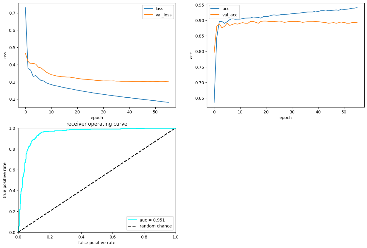
3.7. Plot performance#
Here, we plot the history of the training and the performance in a ROC curve
import matplotlib.pyplot as plt

%matplotlib inline
# plot loss vs epoch
plt.figure(figsize=(15, 10))
ax = plt.subplot(2, 2, 1)
ax.plot(history.history["loss"], label="loss")
ax.plot(history.history["val_loss"], label="val_loss")
ax.legend(loc="upper right")
ax.set_xlabel("epoch")
ax.set_ylabel("loss")

# plot accuracy vs epoch
ax = plt.subplot(2, 2, 2)
ax.plot(history.history["accuracy"], label="acc")
ax.plot(history.history["val_accuracy"], label="val_acc")
ax.legend(loc="upper left")
ax.set_xlabel("epoch")
ax.set_ylabel("acc")

# Plot ROC
Y_predict = model.predict(X_test)
from sklearn.metrics import roc_curve, auc

fpr, tpr, thresholds = roc_curve(Y_test, Y_predict)
roc_auc = auc(fpr, tpr)
ax = plt.subplot(2, 2, 3)
ax.plot(fpr, tpr, lw=2, color="cyan", label="auc = %.3f" % (roc_auc))
ax.plot([0, 1], [0, 1], linestyle="--", lw=2, color="k", label="random chance")
ax.set_xlim([0, 1.0])
ax.set_ylim([0, 1.0])
ax.set_xlabel("false positive rate")
ax.set_ylabel("true positive rate")
ax.set_title("receiver operating curve")
ax.legend(loc="lower right")
plt.show()
32/32 [==============================] - 0s 3ms/step