4. Graph Neural Network (GNN) with PyTorch Geometric#
The contents of this tutorial are heavily adapted from a similar one make by Savannah Thais using tensorflow and keras.
A graph \(G=(N,E)\), comprising of nodes \(N\) and edges \(E\), is a versatile mathematical structure that can represent various data such as molecules, social networks, transportation systems, etc. Nodes and edges may have associated features like geometric or non-geometric information. Graphs can be directed or undirected, and GNNs, with their ability to handle graphs of varying shapes and sizes, are well-suited for diverse applications including High Energy Physics (HEP).
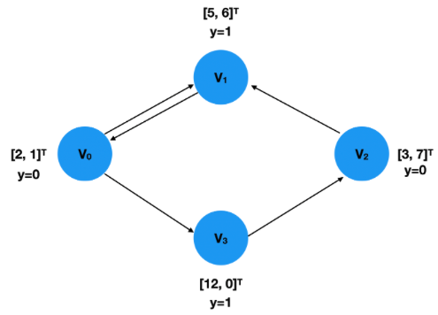
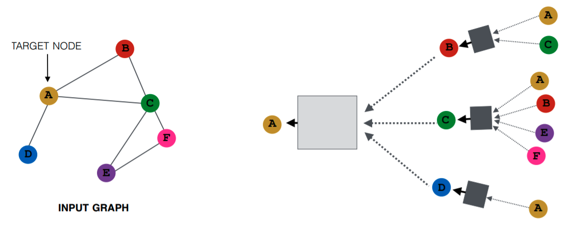
GNNs, particularly Graph Convolutional Networks (GCNs), re-embed graph edges and nodes by applying convolution operations to node neighborhoods, unlike the fixed data tensors used in conventional CNNs. This process, termed as “Message Passing,” constructs messages by combining information from neighboring nodes, then passes them to target nodes to update features. The entire graph is thus transformed, incorporating valuable information within each node. The convolved graph is often further processed for classification or regression on individual elements or the entire graph. This structure can also be applied to update edge features.
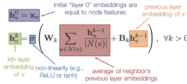
Initial Embedding: Each node \(v\) starts with an initial embedding \(h_v^0\), representing the original node features.
Neighbors: For each node \(v\), the neighboring nodes are represented as \(N(v)\).
Message Construction: To update the embedding of node \(v\), \(h_v^k\), a ‘message’ is constructed through the following steps:
Calculate Average of Neighbors’ Embeddings: Take the average over the current embedding of all neighboring nodes: \(\sum_{u \in N(v)}\frac{h_u^{k-1}}{\text{deg}(v)}\).
Optional Target Node Embedding: Optionally include the current embedding of the target node: \(h_v^{k-1}\).
Apply Function: Use a function \(f\) to combine the above information. In practice, \(f\) is approximated by a matrix (convolution) \(W^k\).
Non-linear Activation: Pass the result through a non-linear activation function to update the target node.
Result: The entire process transforms the graph, updating the node and possibly edge features to include additional useful information. The final embeddings can then be used for further analysis like classification or regression on the graph’s elements or structure.
4.1. Code!#
In this tutorial, we will implement a Graph Neural Network (GNN) using PyTorch Geometric. We’ll perform node classification on the Cora dataset, which consists of scientific publications as nodes and citation links as edges.
The steps in this tutorial include:
Installing PyTorch Geometric
Loading the Cora dataset
Defining the GNN model
Training and evaluating the model
Plotting the training loss and test accuracy
Let’s get started!
# Step 1: Install PyTorch Geometric
!pip install torch_geometric
!pip install torchviz
Requirement already satisfied: torch_geometric in /uscms/home/aaportel/nobackup/mamba/envs/ml/lib/python3.11/site-packages (2.3.1)
Requirement already satisfied: tqdm in /uscms/home/aaportel/nobackup/mamba/envs/ml/lib/python3.11/site-packages (from torch_geometric) (4.65.0)
Requirement already satisfied: numpy in /uscms/home/aaportel/nobackup/mamba/envs/ml/lib/python3.11/site-packages (from torch_geometric) (1.25.1)
Requirement already satisfied: scipy in /uscms/home/aaportel/nobackup/mamba/envs/ml/lib/python3.11/site-packages (from torch_geometric) (1.11.1)
Requirement already satisfied: jinja2 in /uscms/home/aaportel/nobackup/mamba/envs/ml/lib/python3.11/site-packages (from torch_geometric) (3.1.2)
Requirement already satisfied: requests in /uscms/home/aaportel/nobackup/mamba/envs/ml/lib/python3.11/site-packages (from torch_geometric) (2.31.0)
Requirement already satisfied: pyparsing in /uscms/home/aaportel/nobackup/mamba/envs/ml/lib/python3.11/site-packages (from torch_geometric) (3.0.4)
Requirement already satisfied: scikit-learn in /uscms/home/aaportel/nobackup/mamba/envs/ml/lib/python3.11/site-packages (from torch_geometric) (1.3.0)
Requirement already satisfied: psutil>=5.8.0 in /uscms/home/aaportel/nobackup/mamba/envs/ml/lib/python3.11/site-packages (from torch_geometric) (5.9.5)
Requirement already satisfied: MarkupSafe>=2.0 in /uscms/home/aaportel/nobackup/mamba/envs/ml/lib/python3.11/site-packages (from jinja2->torch_geometric) (2.1.3)
Requirement already satisfied: charset-normalizer<4,>=2 in /uscms/home/aaportel/nobackup/mamba/envs/ml/lib/python3.11/site-packages (from requests->torch_geometric) (3.2.0)
Requirement already satisfied: idna<4,>=2.5 in /uscms/home/aaportel/nobackup/mamba/envs/ml/lib/python3.11/site-packages (from requests->torch_geometric) (3.4)
Requirement already satisfied: urllib3<3,>=1.21.1 in /uscms/home/aaportel/nobackup/mamba/envs/ml/lib/python3.11/site-packages (from requests->torch_geometric) (2.0.3)
Requirement already satisfied: certifi>=2017.4.17 in /uscms/home/aaportel/nobackup/mamba/envs/ml/lib/python3.11/site-packages (from requests->torch_geometric) (2023.5.7)
Requirement already satisfied: joblib>=1.1.1 in /uscms/home/aaportel/nobackup/mamba/envs/ml/lib/python3.11/site-packages (from scikit-learn->torch_geometric) (1.3.1)
Requirement already satisfied: threadpoolctl>=2.0.0 in /uscms/home/aaportel/nobackup/mamba/envs/ml/lib/python3.11/site-packages (from scikit-learn->torch_geometric) (3.2.0)
Collecting torchviz
  Downloading torchviz-0.0.2.tar.gz (4.9 kB)
  Preparing metadata (setup.py) ... ?25ldone
?25hRequirement already satisfied: torch in /uscms/home/aaportel/nobackup/mamba/envs/ml/lib/python3.11/site-packages (from torchviz) (2.0.1)
Collecting graphviz (from torchviz)
  Downloading graphviz-0.20.1-py3-none-any.whl (47 kB)
     ━━━━━━━━━━━━━━━━━━━━━━━━━━━━━━━━━━━━━━━ 47.0/47.0 kB 858.8 kB/s eta 0:00:00a 0:00:01
?25hRequirement already satisfied: filelock in /uscms/home/aaportel/nobackup/mamba/envs/ml/lib/python3.11/site-packages (from torch->torchviz) (3.12.2)
Requirement already satisfied: typing-extensions in /uscms/home/aaportel/nobackup/mamba/envs/ml/lib/python3.11/site-packages (from torch->torchviz) (4.7.1)
Requirement already satisfied: sympy in /uscms/home/aaportel/nobackup/mamba/envs/ml/lib/python3.11/site-packages (from torch->torchviz) (1.12)
Requirement already satisfied: networkx in /uscms/home/aaportel/nobackup/mamba/envs/ml/lib/python3.11/site-packages (from torch->torchviz) (3.1)
Requirement already satisfied: jinja2 in /uscms/home/aaportel/nobackup/mamba/envs/ml/lib/python3.11/site-packages (from torch->torchviz) (3.1.2)
Requirement already satisfied: MarkupSafe>=2.0 in /uscms/home/aaportel/nobackup/mamba/envs/ml/lib/python3.11/site-packages (from jinja2->torch->torchviz) (2.1.3)
Requirement already satisfied: mpmath>=0.19 in /uscms/home/aaportel/nobackup/mamba/envs/ml/lib/python3.11/site-packages (from sympy->torch->torchviz) (1.3.0)
Building wheels for collected packages: torchviz
  Building wheel for torchviz (setup.py) ... ?25ldone
?25h  Created wheel for torchviz: filename=torchviz-0.0.2-py3-none-any.whl size=4131 sha256=3593429a9b86799f5b41f3251aeb3d1d55045ea88a70f3ac8410df2eb6c59242
  Stored in directory: /uscms/homes/a/aaportel/.cache/pip/wheels/5a/d0/3f/b7014553eb74f12892b7d9b69c6083044564712d10fde8dfdc
Successfully built torchviz
Installing collected packages: graphviz, torchviz
Successfully installed graphviz-0.20.1 torchviz-0.0.2
4.2. Step 2: Import Libraries and Load Cora Dataset#
We’ll start by importing the necessary libraries and loading the Cora dataset.
import torch
import torch.nn.functional as F
from torch_geometric.nn import GCNConv
from torch_geometric.data import Data
from torch_geometric.datasets import Planetoid
import numpy as np
The Cora dataset consists of 2708 scientific publications classified into one of seven classes. The citation network consists of 5429 links. Each publication in the dataset is described by a 0/1-valued word vector indicating the absence/presence of the corresponding word from the dictionary. The dictionary consists of 1433 unique words.
# Load Cora dataset
dataset = Planetoid(root="/tmp/Cora", name="Cora")
data = dataset[0]
Downloading https://github.com/kimiyoung/planetoid/raw/master/data/ind.cora.x
Downloading https://github.com/kimiyoung/planetoid/raw/master/data/ind.cora.tx
Downloading https://github.com/kimiyoung/planetoid/raw/master/data/ind.cora.allx
Downloading https://github.com/kimiyoung/planetoid/raw/master/data/ind.cora.y
Downloading https://github.com/kimiyoung/planetoid/raw/master/data/ind.cora.ty
Downloading https://github.com/kimiyoung/planetoid/raw/master/data/ind.cora.ally
Downloading https://github.com/kimiyoung/planetoid/raw/master/data/ind.cora.graph
Downloading https://github.com/kimiyoung/planetoid/raw/master/data/ind.cora.test.index
Processing...
Done!
PyTorch Geometric has this nifty class called Data which is used to standardize graph data. You can make your own, but since the sample datasets are already in this format, we won’t go over how to make them here.
data
Data(x=[2708, 1433], edge_index=[2, 10556], y=[2708], train_mask=[2708], val_mask=[2708], test_mask=[2708])
print("node vectors: \n", data.x, "\n")
print("node classes:  \n", data.y, "\n")
print("edge indeces: \n", data.edge_index, "\n\n\n")

print("train_mask: \n", data.train_mask, "\n")
print("val_mask: \n", data.val_mask, "\n")
print("test_mask: \n", data.test_mask, "\n")
node vectors:
 tensor([[0., 0., 0.,  ..., 0., 0., 0.],
        [0., 0., 0.,  ..., 0., 0., 0.],
        [0., 0., 0.,  ..., 0., 0., 0.],
        ...,
        [0., 0., 0.,  ..., 0., 0., 0.],
        [0., 0., 0.,  ..., 0., 0., 0.],
        [0., 0., 0.,  ..., 0., 0., 0.]])

node classes:
 tensor([3, 4, 4,  ..., 3, 3, 3])

edge indeces:
 tensor([[   0,    0,    0,  ..., 2707, 2707, 2707],
        [ 633, 1862, 2582,  ...,  598, 1473, 2706]])


train_mask:
 tensor([ True,  True,  True,  ..., False, False, False])

val_mask:
 tensor([False, False, False,  ..., False, False, False])

test_mask:
 tensor([False, False, False,  ...,  True,  True,  True])
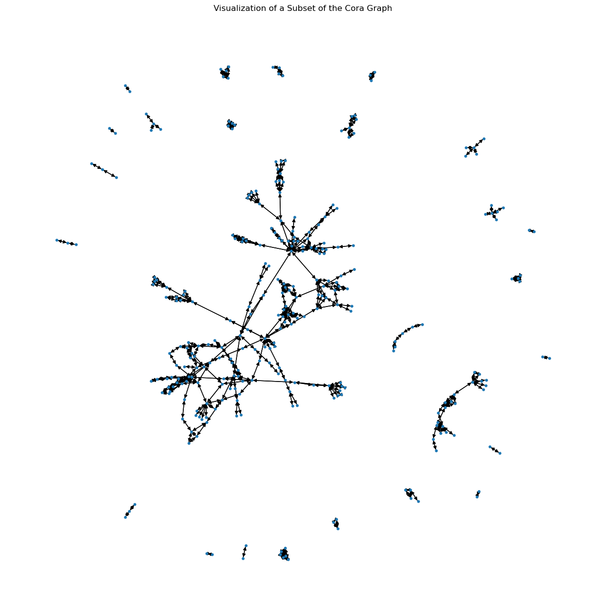
We can also visualize the dataset using networkx:
import networkx as nx
import matplotlib.pyplot as plt

# Convert to networkx graph
G = nx.DiGraph()
for i, j in zip(*data.edge_index):
    G.add_edge(i.item(), j.item())

# Draw a subset of the graph (e.g., first 300 nodes)
subset_nodes = list(G.nodes)[:300]
subset_graph = G.subgraph(subset_nodes)

plt.figure(figsize=(12, 12))
nx.draw(subset_graph, with_labels=False, node_size=10)
plt.title("Visualization of a Subset of the Cora Graph")
plt.show()
4.3. Step 3: Define the GNN Model#
Next, we’ll define the GNN model, consisting of two GCN convolution layers.
# Define GNN model
class GNN(torch.nn.Module):
    def __init__(self, hidden_channels):
        super(GNN, self).__init__()
        self.conv1 = GCNConv(dataset.num_node_features, hidden_channels)
        self.conv2 = GCNConv(hidden_channels, dataset.num_classes)

    def forward(self, x, edge_index):
        x = self.conv1(x, edge_index)
        x = x.relu()
        x = F.dropout(x, p=0.1, training=self.training)
        x = self.conv2(x, edge_index)
        return x
4.4. Step 4: Training and Evaluation#
Now, we’ll train the GNN model and evaluate its performance.
# Training and evaluation
device = torch.device("cuda" if torch.cuda.is_available() else "cpu")
model = GNN(hidden_channels=16).to(device)
data = data.to(device)
optimizer = torch.optim.Adam(model.parameters(), lr=0.01, weight_decay=5e-4)
import matplotlib.pyplot as plt


# Lists to store loss and accuracy over time
train_loss_history = []
test_accuracy_history = []


def train():
    model.train()
    optimizer.zero_grad()
    out = model(data.x, data.edge_index)
    loss = F.cross_entropy(out[data.train_mask], data.y[data.train_mask])
    loss.backward()
    optimizer.step()
    return loss.item()


def test():
    model.eval()
    out = model(data.x, data.edge_index)
    pred = out.argmax(dim=1)
    correct = pred[data.test_mask] == data.y[data.test_mask]
    acc = int(correct.sum()) / int(data.test_mask.sum())
    return acc


for epoch in range(300):
    loss = train()
    train_loss_history.append(loss)
    accuracy = test()
    test_accuracy_history.append(accuracy)
    if epoch % 10 == 0:
        print(f"Epoch: {epoch:03d}, Loss: {loss:.4f}, Accuracy: {accuracy:.4f}")

print("Test Accuracy:", test())
Epoch: 000, Loss: 1.9487, Accuracy: 0.5430
Epoch: 010, Loss: 0.5831, Accuracy: 0.7720
Epoch: 020, Loss: 0.1152, Accuracy: 0.7910
Epoch: 030, Loss: 0.0307, Accuracy: 0.7810
Epoch: 040, Loss: 0.0135, Accuracy: 0.7890
Epoch: 050, Loss: 0.0162, Accuracy: 0.7860
Epoch: 060, Loss: 0.0153, Accuracy: 0.7900
Epoch: 070, Loss: 0.0202, Accuracy: 0.7940
Epoch: 080, Loss: 0.0180, Accuracy: 0.7970
Epoch: 090, Loss: 0.0184, Accuracy: 0.7970
Epoch: 100, Loss: 0.0168, Accuracy: 0.7960
Epoch: 110, Loss: 0.0176, Accuracy: 0.8010
Epoch: 120, Loss: 0.0160, Accuracy: 0.7990
Epoch: 130, Loss: 0.0154, Accuracy: 0.8000
Epoch: 140, Loss: 0.0150, Accuracy: 0.8040
Epoch: 150, Loss: 0.0125, Accuracy: 0.8050
Epoch: 160, Loss: 0.0141, Accuracy: 0.8020
Epoch: 170, Loss: 0.0121, Accuracy: 0.8080
Epoch: 180, Loss: 0.0136, Accuracy: 0.7990
Epoch: 190, Loss: 0.0132, Accuracy: 0.8070
Epoch: 200, Loss: 0.0102, Accuracy: 0.8030
Epoch: 210, Loss: 0.0115, Accuracy: 0.7990
Epoch: 220, Loss: 0.0117, Accuracy: 0.8060
Epoch: 230, Loss: 0.0118, Accuracy: 0.8010
Epoch: 240, Loss: 0.0101, Accuracy: 0.8080
Epoch: 250, Loss: 0.0093, Accuracy: 0.8070
Epoch: 260, Loss: 0.0120, Accuracy: 0.8070
Epoch: 270, Loss: 0.0093, Accuracy: 0.8080
Epoch: 280, Loss: 0.0114, Accuracy: 0.8030
Epoch: 290, Loss: 0.0094, Accuracy: 0.8050
Test Accuracy: 0.806
4.5. Step 5: Plotting Loss and Accuracy#
Finally, we’ll visualize the training loss and test accuracy using Matplotlib.
# Plotting loss and accuracy
fig, (ax1, ax2) = plt.subplots(1, 2, figsize=(15, 5))

ax1.plot(train_loss_history)
ax1.set_xlabel("Epochs")
ax1.set_ylabel("Loss")
ax1.set_title("Training Loss")

ax2.plot(test_accuracy_history)
ax2.set_xlabel("Epochs")
ax2.set_ylabel("Accuracy")
ax2.set_title("Test Accuracy")

plt.show()
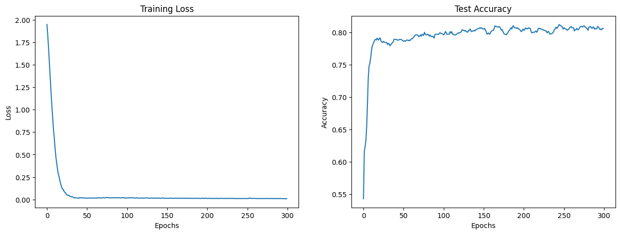
4.6. Conclusion#
In this tutorial, we implemented a GNN model to classify scientific publications in the Cora dataset. We trained the model and visualized the training progress. Experiment with different hyperparameters and architectures to see how the performance changes!