7. Generative Adversarial Networks with Keras and MNIST

Author: Raghav Kansal

Code adapted from this repo.

7.1. Overview

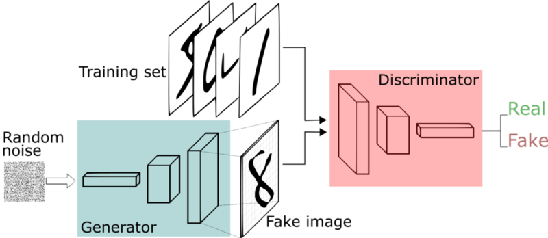
A GAN consists of two individual networks: a discriminator and a generator. We will implement both in Keras and see how to train them to reproduce handwritten digits from the MNIST dataset.

GANs generally work by pitting the two networks against each other. The goal of the generator is to learn the data distribution, while the goal of the discriminator is to be able to distinguish between the fake data produced by the generator and the real data from the training set. They are trained in turn: the generator takes as input random samples from a latent space and outputs fake data, its target being to fool the discriminator into classifying the fake data is real; the discriminator takes as input both real and fake data and tries to classify it correctly as real or fake. Ultimately after training them both fully the hope is that the generator is able to produce realistic looking data.

We can think of this as a feedback system, or as a ‘minimax’ two-player game. Training GANs is notoriously difficult, precisely because we need to train these two, inherently adversarial, networks simultaneously.

7.1.1. Importing and preprocessing our data

import numpy as np
from tqdm.notebook import tqdm
import matplotlib.pyplot as plt

from tensorflow.keras.layers import Input, Reshape, Dense, Dropout, LeakyReLU
from tensorflow.keras.models import Model, Sequential
from tensorflow.keras.datasets import mnist

# temporarily importing legacy optimizer because of
# https://github.com/keras-team/keras-io/issues/1241#issuecomment-1442383703
from tensorflow.keras.optimizers.legacy import Adam
from tensorflow.keras import backend as K
from tensorflow.keras import initializers
import tensorflow as tf

np.random.seed(1000)

latent_dim = 100  # Our latent space will consist of 100 independent continuous variables

# we'll be plotting 10 generated images with the same input sample each epoch
im_examples = 10
im_noise = np.random.normal(0, 1, size=[10, latent_dim])

# normalizing MNIST data and converting image to vector
(X_train, y_train), (X_test, y_test) = mnist.load_data()
X_train = (X_train.astype(np.float32) - 127.5) / 127.5
X_train = X_train.reshape(60000, 784)

# We'll use the Adam optimization algorithm (https://arxiv.org/pdf/1412.6980.pdf)
adam = Adam(learning_rate=0.0002, beta_1=0.5)

7.1.2. Defining our model

As explained in the overview, we need to define a generator network and a discriminator network. Note that ultimately both are trying to solve a 2-class classification problem (real or fake) so canonically we use the binary cross entropy as their loss function. A variant of the GAN, the Least Squares GAN, uses the mean squared error instead and can often be more effective.

The generator will take a random sample from our latent space as its input, then after four fully connected layers output a MNIST data sample:

generator = Sequential()
generator.add(
    Dense(256, input_dim=latent_dim, kernel_initializer=initializers.RandomNormal(stddev=0.02))
)
generator.add(LeakyReLU(0.2))
generator.add(Dense(512))
generator.add(LeakyReLU(0.2))
generator.add(Dense(1024))
generator.add(LeakyReLU(0.2))
generator.add(Dense(784, activation="tanh"))
generator.compile(loss="binary_crossentropy", optimizer=adam)

The discriminator takes a MNIST, or fake MNIST data sample after four fully connected layers outputs whether it thinks the sample is real or fake. Generally, unless their is a reason not to, we choose the generator and discriminator architectures to be mirror images.

discriminator = Sequential()
discriminator.add(
    Dense(1024, input_dim=784, kernel_initializer=initializers.RandomNormal(stddev=0.02))
)
discriminator.add(LeakyReLU(0.2))
discriminator.add(Dropout(0.3))  # dropout in the discriminator to avoid overfitting
discriminator.add(Dense(512))
discriminator.add(LeakyReLU(0.2))
discriminator.add(Dropout(0.3))
discriminator.add(Dense(256))
discriminator.add(LeakyReLU(0.2))
discriminator.add(Dropout(0.3))
discriminator.add(Dense(1, activation="sigmoid"))
discriminator.compile(loss="binary_crossentropy", optimizer=adam)

Finally the combined network, which feeds a random sample from the latent space into the generator and tests the output using the discriminator. As you will see below, this will only be used to train the generator, which is why we set the discriminator to not be trainable before compiling the network.

# Combined network
discriminator.trainable = False
gan_input = Input(shape=(latent_dim,))
x = generator(gan_input)
gan_output = discriminator(x)
gan = Model(inputs=gan_input, outputs=gan_output)
gan.compile(loss="binary_crossentropy", optimizer=adam)

# For plotting the losses for both networks at the end
def plotLoss():
    plt.figure(figsize=(10, 8))
    plt.plot(dLosses, label="Discriminitive loss")
    plt.plot(gLosses, label="Generative loss")
    plt.xlabel("Epoch")
    plt.ylabel("Loss")
    plt.legend()
    plt.show()

# We'll plot a sample of the generated images after each epoch
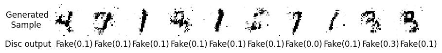
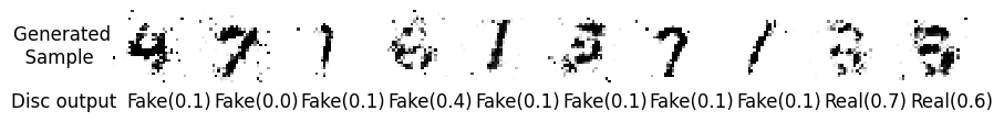
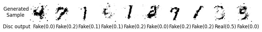
def plotGeneratedImages():
    dim = (1, im_examples + 1)

    generated_images = generator.predict(im_noise, verbose=0)
    disc_output = discriminator.predict(generated_images, verbose=0)
    generated_images = generated_images.reshape(im_examples, 28, 28)

    plt.figure(figsize=(im_examples + 1, im_examples + 1))

    plt.subplot(dim[0], dim[1], 1)
    plt.imshow(np.zeros((28, 28)), cmap="gray_r")
    plt.axis("off")
    plt.text(-5, 20, "Generated \n  Sample", fontsize=12)
    plt.text(-6, 37, "Disc output", fontsize=12)

    for i in range(generated_images.shape[0]):
        plt.subplot(dim[0], dim[1], i + 2)
        plt.imshow(generated_images[i], interpolation="nearest", cmap="gray_r")
        val = (
            "Real(%.1f)" % disc_output[i] if disc_output[i] > 0.5 else "Fake(%.1f)" % disc_output[i]
        )
        plt.text(5, 37, val, fontsize=12)
        plt.axis("off")

    plt.show()

7.1.3. Training

In each iteration we train the discriminator and generator in turn. Typically we start with the discriminator, which takes a batch of real images and a batch of fake images and is trained to classify them correctly. Then we train the generator to try to produce images which the discriminator will classify as real.

def train(epochs=1, batch_size=128):
    num_batches = int(X_train.shape[0] / batch_size)
    plotGeneratedImages()

    for e in range(1, epochs + 1):
        print("-" * 15, "Epoch %d" % e, "-" * 15)
        for _ in tqdm(range(num_batches)):
            # Sample random noise from our latent space
            noise = np.random.normal(0, 1, size=[batch_size, latent_dim])
            # Sample random images from the real dataset
            image_batch = X_train[np.random.randint(0, X_train.shape[0], size=batch_size)]

            # Generate fake MNIST images
            generated_images = generator.predict(noise, verbose=0)
            X = np.concatenate([image_batch, generated_images])

            # Labels for generated and real data - the correct labels are 1s for the real and 0s for fake images
            yDis = np.zeros(2 * batch_size)
            yDis[:batch_size] = 0.9  # labeling as 0.9 instead of 1 is known as 'label smoothing'.
            # Essentially we are penalizing the discriminator for being too sure about the real images
            # We are doing this here because without it the discriminator was working too well and not letting the generator improve.

            # Training discriminator. We have to tell Keras when the discriminator is or isn't being trained
            discriminator.trainable = True
            dloss = discriminator.train_on_batch(X, yDis)

            # Training the generator to have the discriminator classify its produced images as real i.e. output 1s.
            noise = np.random.normal(0, 1, size=[batch_size, latent_dim])
            yGen = np.ones(batch_size)
            discriminator.trainable = False
            gloss = gan.train_on_batch(noise, yGen)

        # Store loss of most recent batch from this epoch
        dLosses.append(dloss)
        gLosses.append(gloss)

        plotGeneratedImages()

        if e % 10 == 0:
            plotLoss()

Finally, running the code:

dLosses = []
gLosses = []

train(5, 128)

--------------- Epoch 1 ---------------

--------------- Epoch 2 ---------------

--------------- Epoch 3 ---------------

--------------- Epoch 4 ---------------

--------------- Epoch 5 ---------------

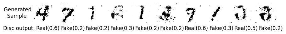
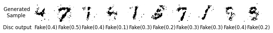
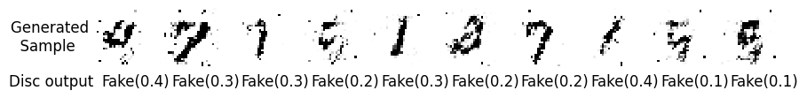
We can see the generated images improved each epoch. Eventually, if training goes well, the generator will converge to realistic looking data samples. GANs have worked remarkably well on a number of datasets. This blog goes through some interesting examples, such as faces:

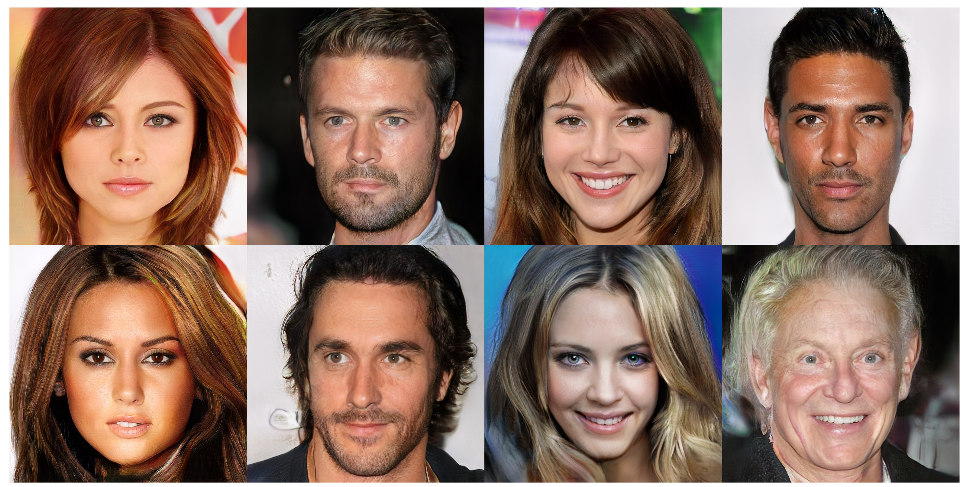All artifically produced with a GAN.

Several groups at CERN are also experimenting with GANs for fast data simulation: see GANs section in the HEP ML Living Review.

Finally, for those interested in training your own GAN, check out some common variants such as the WGAN and the LSGAN which can be more effective.