Overview

Teaching: min
Exercises: min

Questions

Objectives

Analyzing a single count using RooFit/RooStats

Mathematical Background 1

The goal of this exercise is to infer a value for the signal strength parameter $\mu$, defined by

\[n = \mu s + b_{ZZ} + b_{ZX}\]

where $s$ and $b_{*} $ are the mean and background counts, respectively. We shall use lower case to denote parameters, that is, the unknowns, while an estimate of a parameter, a known, is denoted by the parameter decorated with a hat, e.g. $\hat{b}_{ZZ}$ is an estimate of $b_{ZZ}$

Observations, also known, are denoted with upper case variables. This is shown in the table below.

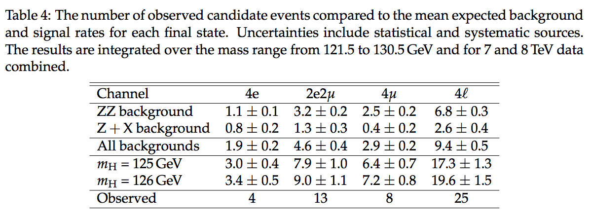
knowns	unknowns
$N$	$n$
$\hat{b}_{ZZ} \pm \delta b_{ZZ}$	$b_{ZZ}$
$\hat{b}_{ZX} \pm \delta b_{ZX}$	$b_{ZX}$
$\hat{s} \pm \delta s$	$s$
	$\mu$

According to Table 4, the total observed number of 4-lepton events is $N=25$. Since this number is known, we are certain about its value! On the other hand, the expected count $n$ is unknown. Consequently, we are uncertain about its value. Therefore, $25\pm5$ is a statement about $n$ not about 25.

The likelihood

We take the likelihood associated with the observed count to be

\[\mathcal{L}(n) = {\rm Poisson}(N;n) = \exp(-n)\; n^N / N!\]

What about that for $\hat{b}_{*}$ and $\hat{s}$? If we were performing Bayesian calculations only, we would simply write down a prior density for both parameters, say a gamma density. However, we also want to perform frequentist calculations, which do not use priors. So, somehow, we need to mock up likelihoods for the background and the signal estimates.

An obvious choice is to model the likelihoods with Gaussians (as in exercise_1b. But, since we know that the signal and background, in this problem, cannot be negative we need to work a bit harder. A standard way to proceed is to model each estimate as an (effective) Poisson count, $Q$ that has been scaled by a factor $q$, for example,

\[\hat{b} = Q/q\] \[\delta b = \sqrt{Q}/q\]

Given this plausible ansatz, we can invert it to arrive at the effective count and scale factor,

\[Q = (\hat{b}/ \delta b)^2\] \[q = Q/\hat{b}\]

We can now model the likelihoods for signal and background as Poisson distributions (continued to non-integral counts). Therefore, the likelihood for this problem is taken to be

\[L(μ,s,b_{ZZ},b_{ZX})={\rm Poisson}(N;\mu s+b_{ZZ}+b_{ZX})\] \[\times \; {\rm Poisson}(B_{ZZ};\tau_{ZZ} b_{ZZ})\] \[\times \;{\rm Poisson}(B_{ZX};\tau_{ZX} b_{ZX})\] \[\times \;{\rm Poisson}(S;\tau_{ss})\]

where

\[B_j=(\hat{b}_j/δb_j)^2,\quad j=ZZ,ZX,\] \[\tau_j = \hat{b}_j / \delta b_j^2 ,\] \[S = (\hat{s} / \delta s)^2,\] \[\tau_s = \hat{s} / \delta s^2,\]

are the effective counts and scale factors for the $ZZ$ and $Z+X$ backgrounds and the signal. Note that in this context, $s$ and $b_j$ are nuisance parameters. Therefore, in order to make inferences about the signal strength, we need to reduce the likelihood $\mathcal{L}(μ,s,b_{ZZ},b_{ZX})$ to a function of $μ$ only. This can be done either by

• profiling, that is replacing $s$ and $b_j$ with their best fit values $\hat{s}(μ)$ and $\hat{b}_j(μ)$ for a given value of $μ$, or by
• marginalization, that is, integrating the likelihood times a prior with respect to $s$ and $b_j$. A uniform prior in $s$ and $b_j$ is used.

Mathematical Background 2 (rephrased)

We will be using this popular model a lot in this exercise. It is simple, and it is sufficient to showcase most of the components of a statistical analysis for a CMS measurement. We will consider a common case of a counting experiment: a number of events is observed in data, some of which may be signal events and the rest background. Event counts are expected to be distributed according to the Poisson distribution. We have some idea about the background yield, and we want to find a confidence interval for the mean signal, that is, for the Poisson mean for the signal. We can write down the statistical model for the count $X$ as

\[p(X|\mu) = \frac{\mu^X e^{-\mu}}{X!} , \quad \mu = \mu_{\rm SIG} + \mu_{\rm BG}\]

When we set $X = N$ in the statistical model, we arrive at the likelihood function, which is the basis for the statistical analysis. Note: it is important to distinguish the likelihood and the statistical model. The statistical model is the probability (or probability density) for observing some data for given values of the model parameters, while the likelihood is a function of the model parameters for a given dataset. So you may think of likelihood as the statistical model computed for specific data. But the Likelihood is not a statistical model, that is, a probabilty model, for the model parameters. In case of the counting experiment, the likelihood is obtained by substituting $X$ with the observed event count $(N)$:

\[\mathcal{L}(N|\mu) = \frac{\mu^N e^{-\mu}}{N!} \ \cdot \mathcal{L}(\mu_{\rm BG})\]

Here $\mathcal{L}(\mu_{\rm BG})$ represents the piece of the likelihood that describes our knowledge about the background. (Usually, this is a likelihood of a previous or an adjacent calibration experiment.)

We want to compute a confidence interval for $μ_{\rm SIG}$.

Note that this model is exactly what is used in the notorious roostats_cl95.C routine.

The task is to analyze the data in the last column of the Table 4, using RooFit/RooStats; in particular, to compute a confidence interval for the signal strength parameter $μ$, defined by

where $s$ and $b_{j}, \ j = ZZ, ZX $ are the expected, that is mean signal background counts, respectively, given the associated estimates $\hat{s} \pm \delta s$ and $\hat{b} \pm \delta b$. In this exercise, we shall assume that the signal and background estimates are statistically independent. (Lack of correlation is a weaker condition: two quantities $X$ and $Y$ can be uncorrelated yet be statistically dependent, that is, their joint probability density $p(X,Y)$ cannot be written as $p(X)p(Y)$.)

The notebook exercise_1a.ipynb

• creates a RooWorkspace
• creates the model parameters
• creates a model (a pdf in RooFit jargon) equal to the product of four Poisson distributions, one for the observed count $N$, one for each of the effective background counts $B_{ZZ}$ and $B_{ZX}$, and one for the effective signal count $S$
• writes out the workspace to file single_count.root
• reads in the workspace
• finds the MLE of $μ$, and
• computes a confidence interval, a credible interval, and an upper limit on $μ$.

The end of the output should look like:

Floating Parameter    FinalValue +/-  Error   
  --------------------  --------------------------
                  b_zx    2.6001e+00 +/-  3.00e-01
                  b_zz    6.8002e+00 +/-  3.00e-01
                    mu    9.0151e-01 +/-  2.96e-01
                     s    1.7299e+01 +/-  1.30e+00

compute interval using profile likelihood
   PL 68.3% CL interval = [ 0.63,  1.22]
   PL 95.0% upper limit =  1.46

compute interval using Bayesian calculator
   Bayes 68.3% CL interval = [ 0.68,  1.28]
      ...be patient...!
   Bayes 95.0% upper limit =  1.51

Info in : file ./fig_PL.png has been created
Info in : file ./fig_Bayes.png has been created

and two plots should appear. Here are some suggested tasks.

Suggestions

• Repeat the calculation for $m_H = 126\textrm{GeV}$.

Hint

You can find the $m_H = 126\textrm{GeV}$ predictions in the comments at the top of exercise_1a.ipynb

• Replace the signal and background likelihoods by Gaussians and re-rerun. Do so before looking at exercise_1b! (See code snippet below).

  wspace.factory('Gaussian::pB_zz(b_hat_zz, b_zz, db_zz)')
  wspace.factory('Gaussian::pB_zx(b_hat_zx, b_zx, db_zx)')
  wspace.factory('Gaussian::pS(s_hat, s, ds)')
  

Hint

We want to use Gaussians for the signal and background likelihoods as defined above. To make exercise_1.ipynb execute the above lines of code, “pdfs” needs to be redefined as follows:

pdfs = [('Poisson', 'pN',    '(N, n)'),
        ('Gaussian', 'pB_zz', '(b_hat_zz, b_zz, db_zz)'), 
        ('Gaussian', 'pB_zx', '(b_hat_zx, b_zx, db_zx)'),
        ('Gaussian', 'pS',    '(s_hat,    s,     ds)')]

Key Points