Introduction
Overview
Teaching: 10 min
Exercises: 0 minQuestions
What are the goals of a statistical analysis?
Objectives
Learn a few statistical concepts and their relationship to probability.
It is hardly possible today to avoid the use of statistical analysis. Consider the standard problem of measuring (or as statisticians say, estimating) the signal $s$ given the observation of a single count $N$ and given a background estimate $B\pm \delta B$. The obvious answer, which requires no fancy statistics, is $\hat s = N−B$ . But the estimate $\hat s$ is, of course, not enough. We need somehow to quantify its accuracy. It is generally accepted that a good way to do this is to compute an interval $[\underline{s}(N), \overline{s}(N)]$. But that too is not enough! We must also associate some measure (other than its width) to the interval. Why? So that we may compare intervals. Generally, one considers a shorter interval to be more accurate than a longer one, but it is only possible to make a meaningful statement when both are compared using the same value of the measure. The measure we use is probability. The probability can be interpreted as the fraction of intervals (not necessarily pertaining to the same measured quantity) that bracket the true (but generally unknown) value of that quantity; this is an example of the frequentist interpretation of probability, which in this context is called the confidence level (CL) associated with the confidence intervals. (Note: intervals plural; the CL is a property of the ensemble in which the interval is presumed to reside. Consequently, if one changes the parent ensemble then, in general, the CL will change.) Or, the probability can be interpreted as the degree of belief to be assigned to the statement $s \in [\underline{s}, \overline{s}]$; this is the Bayesian interpretation of probability, which in the present context is called a credible (or credibility) level (CL) associated with the given credible interval.
Given the ubiquity of statistical procedures in our field, tools have been created to help perform them correctly. In these exercises, you will learn how to use the statistical modeling toolkit RooFit and the associated statistical analysis toolkit RooStats to perform some standard, but very widely used, statistical procedures, including fitting, estimating (i.e., measuring) parameters, computing intervals, and setting limits. You will also learn how to use the tool combine, which, as its name suggests, can be used to perform statistical analyses of multiple results.
In order to focus on the essentials, and yet have realistic examples, exercises 1, 2, and 3 use the following data
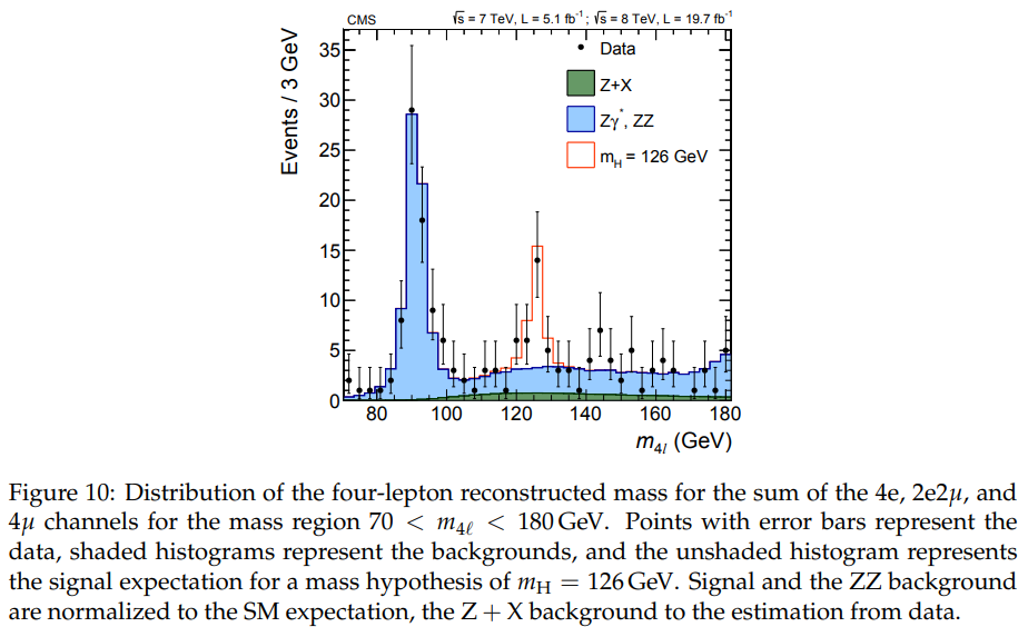
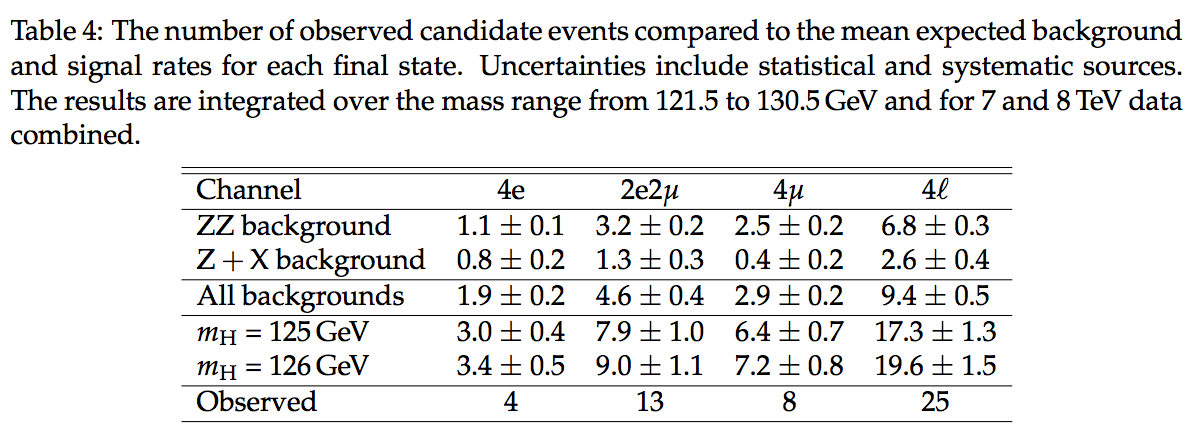
taken from the CMS $H \to ZZ \to 4\ell$ Run I summary paper ( Measurement of the properties of the Higgs boson in the four-lepton final states, Phys. Rev. D 89 092007 (2014)).
Key Points
Exercise 0
Overview
Teaching: min
Exercises: minQuestions
Objectives
A very short Python/PyROOT/RooFit tutorial
Mathematical Background
The notebook
\[f(x;\theta)=a\exp(-x/b)/b+(1-a)\exp(-x/c)/c,\quad\theta=a,b,c\] \[\int f(x;\theta)\; dx=1\]exercise_0.ipynbgenerates data from the modeland fits the same model to the data using both un-binned and binned fits. In both cases, the famed minimizer
\[l(\theta) = - \ln \mathcal{L}(\theta)\]Minuitfrom CERN is used to minimize the negative log-likelihood (which is equivalent to maximizing the likelihood),with respect to the parameters $\theta$ of the model. For the un-binned fit, the likelihood (that is, the pdf evaluated at the observed data) is
\[\mathcal{L}(\theta) = \prod_{i=1}^T f(x_i; \theta)\]where $T$ is the number of data. For the binned fit, the likelihood is the multinomial
\[\mathcal{L}(\theta) = \prod_{i=1}^M p_i^{N_i}\]where $M$ is the number of bins, $N_i$ the count in the $i^{\text{th}}$ bin,
\[p_i = \frac{n_i}{\sum_{j=1}^M n_j}\]and the expected count in the $i^{\text{th}}$ bin is
\[n_i = T \int_{\text{bin}_i} f(x;\theta)\; dx\]Quality of binned fit
The quality of the binned fit is assessed using two goodness-of-fit (gof) measures
\[X = \sum_{i=1}^M \frac{(N_i - n_i)^2}{n_i}\]and
\[Y = -2 \sum_{i=1}^M N_i \ln (n_i / N_i)\]According to Wilks theorem (1938), if the hypothesis $H_0 : \theta= \theta_0$ is true, and $\theta_0$ does not lie on the boundary of the parameter space (plus some other mild conditions), then asymptotically (that is, as $T\to \infty$) both measures have a $\chi^2_K$ distribution of $K$ degrees of freedom. For a multinomial distribution with $M$ bins and $P$ fitted parameters $K=M−1−P$. The true hypothesis $H_0$ is approximated by setting $\theta_0=\hat{\theta}$, the best fit values (that is, maximum likelihood estimates (MLE)) of $\theta$.
If $X \approx Y \approx K$, we may conclude that we have no grounds for rejecting the hypothesis $H_0$. A probabilistic way to say the same thing is to compute a p-value, defined by
\[\text{p-value} = {\rm Pr}(X' > X | H_0)\]under the assumption that $H_0$ is true and reject the hypothesis if the p-value is judged to be too small. The intuition here is that if we observe a gof measure that is way off in the tail of the distribution of $X$, then either a rare fluctuation has occurred or the hypothesis $H_0$ is false. It is a matter of judgment and, or, convention which conclusion is to be adopted.
All of this, of course, depends on the validity of the asymptotic approximation. One way to check whether the approximation is reasonable is to compare the measures $X$ and $Y$, or, equivalently, their associated p-values. Should they turn out to be about the same, then we can happily conclude that the land of Asymptotia is in sight!
In this exercise you will learn how to use RooFit (via the Python/ROOT interface, PyROOT) to fit functions to data. As an example, the notebook exercise_0.ipynb generates “pseudo-data” from a given model, and then fits that pseudo-data using the same functional form. The first part of the exercise consists simply of running the notebook exercise_0.ipynb, reading through the program, and trying to understand what it is doing.
This program fits a double exponential to the unbinned pseudo-data. The pseudo-data are then binned and a binned fit is performed using a multinomial likelihood. Finally, two goodness-of-fit (gof) measures are calculated and converted into p-values. (See mathematical background for details.) The last output you should see should look something like
Info in : file ./fig_binnedFit.png has been created
================================================================================

            binlow count       mean
    1        0.000   109      103.4
    2        1.333    70       71.1
    3        2.667    48       50.6
    4        4.000    33       37.2
    5        5.333    33       28.3
    6        6.667    18       22.2
    7        8.000    16       17.8
    8        9.333    16       14.6
    9       10.667    17       12.1
   10       12.000     8       10.2
   11       13.333     8        8.7
   12       14.667     9        7.4
   13       16.000     5        6.3
   14       17.333     6        5.4
   15       18.667     4        4.7
================================================================================
Int p(x|xi) dx = 400.0

ChiSq/ndf =    6.0/10 (using X)
p-value   =    0.8153

ChiSq/ndf =    7.2/10 (using Y)
p-value   =    0.7033
and two plots should appear, then disappear. Read through the notebook exercise_0.ipynb and try to understand what it is doing. Feel free to play around with the notebook. Check the suggestions below for examples of things you can change.
Suggestions
- Change the number of pseudo-data events to generate and re-run the fit.
- Change the number of bins and re-run the fit.
- Add a new function (for example, a Gaussian + an exponential) to models.cc, modify the notebook to use it by modifying the code highlighted below, and re-run.
gROOT.ProcessLine(open('models.cc').read())
from ROOT import dbexp
wspace.factory('GenericPdf::model("dbexp(x,a,b,c)", {x,a,b,c})')
If you add more parameters, you’ll need to modify the code block:
# The parameters of the model are a, b, c
wspace.factory('a[0.4, 0.0,   1.0]')
wspace.factory('b[3.0, 0.01, 20.0]')
wspace.factory('c[9.0, 0.01, 20.0]')
parameters = ['a', 'b', 'c']

# NUMBER OF PARAMETERS
P = len(parameters)
Key Points
Exercise 1
Overview
Teaching: min
Exercises: minQuestions
Objectives
Analyzing a single count using RooFit/RooStats
Mathematical Background 1
The goal of this exercise is to infer a value for the signal strength parameter $\mu$, defined by
\[n = \mu s + b_{ZZ} + b_{ZX}\]where $s$ and $b_{*} $ are the mean and background counts, respectively. We shall use lower case to denote parameters, that is, the unknowns, while an estimate of a parameter, a known, is denoted by the parameter decorated with a hat, e.g. $\hat{b}_{ZZ}$ is an estimate of $b_{ZZ}$
Observations, also known, are denoted with upper case variables. This is shown in the table below.
knowns unknowns $N$ $n$ $\hat{b}_{ZZ} \pm \delta b_{ZZ}$ $b_{ZZ}$ $\hat{b}_{ZX} \pm \delta b_{ZX}$ $b_{ZX}$ $\hat{s} \pm \delta s$ $s$ $\mu$ According to Table 4, the total observed number of 4-lepton events is $N=25$. Since this number is known, we are certain about its value! On the other hand, the expected count $n$ is unknown. Consequently, we are uncertain about its value. Therefore, $25\pm5$ is a statement about $n$ not about 25.
The likelihood
We take the likelihood associated with the observed count to be
\[\mathcal{L}(n) = {\rm Poisson}(N;n) = \exp(-n)\; n^N / N!\]What about that for $\hat{b}_{*}$ and $\hat{s}$? If we were performing Bayesian calculations only, we would simply write down a prior density for both parameters, say a gamma density. However, we also want to perform frequentist calculations, which do not use priors. So, somehow, we need to mock up likelihoods for the background and the signal estimates.
An obvious choice is to model the likelihoods with Gaussians (as in
\[\hat{b} = Q/q\] \[\delta b = \sqrt{Q}/q\]exercise_1b. But, since we know that the signal and background, in this problem, cannot be negative we need to work a bit harder. A standard way to proceed is to model each estimate as an (effective) Poisson count, $Q$ that has been scaled by a factor $q$, for example,Given this plausible ansatz, we can invert it to arrive at the effective count and scale factor,
\[Q = (\hat{b}/ \delta b)^2\] \[q = Q/\hat{b}\]We can now model the likelihoods for signal and background as Poisson distributions (continued to non-integral counts). Therefore, the likelihood for this problem is taken to be
\[L(μ,s,b_{ZZ},b_{ZX})={\rm Poisson}(N;\mu s+b_{ZZ}+b_{ZX})\] \[\times \; {\rm Poisson}(B_{ZZ};\tau_{ZZ} b_{ZZ})\] \[\times \;{\rm Poisson}(B_{ZX};\tau_{ZX} b_{ZX})\] \[\times \;{\rm Poisson}(S;\tau_{ss})\]where
\[B_j=(\hat{b}_j/δb_j)^2,\quad j=ZZ,ZX,\] \[\tau_j = \hat{b}_j / \delta b_j^2 ,\] \[S = (\hat{s} / \delta s)^2,\] \[\tau_s = \hat{s} / \delta s^2,\]are the effective counts and scale factors for the $ZZ$ and $Z+X$ backgrounds and the signal. Note that in this context, $s$ and $b_j$ are nuisance parameters. Therefore, in order to make inferences about the signal strength, we need to reduce the likelihood $\mathcal{L}(μ,s,b_{ZZ},b_{ZX})$ to a function of $μ$ only. This can be done either by
- profiling, that is replacing $s$ and $b_j$ with their best fit values $\hat{s}(μ)$ and $\hat{b}_j(μ)$ for a given value of $μ$, or by
- marginalization, that is, integrating the likelihood times a prior with respect to $s$ and $b_j$. A uniform prior in $s$ and $b_j$ is used.
Mathematical Background 2 (rephrased)
We will be using this popular model a lot in this exercise. It is simple, and it is sufficient to showcase most of the components of a statistical analysis for a CMS measurement. We will consider a common case of a counting experiment: a number of events is observed in data, some of which may be signal events and the rest background. Event counts are expected to be distributed according to the Poisson distribution. We have some idea about the background yield, and we want to find a confidence interval for the mean signal, that is, for the Poisson mean for the signal. We can write down the statistical model for the count $X$ as
\[p(X|\mu) = \frac{\mu^X e^{-\mu}}{X!} , \quad \mu = \mu_{\rm SIG} + \mu_{\rm BG}\]When we set $X = N$ in the statistical model, we arrive at the likelihood function, which is the basis for the statistical analysis. Note: it is important to distinguish the likelihood and the statistical model. The statistical model is the probability (or probability density) for observing some data for given values of the model parameters, while the likelihood is a function of the model parameters for a given dataset. So you may think of likelihood as the statistical model computed for specific data. But the Likelihood is not a statistical model, that is, a probabilty model, for the model parameters. In case of the counting experiment, the likelihood is obtained by substituting $X$ with the observed event count $(N)$:
\[\mathcal{L}(N|\mu) = \frac{\mu^N e^{-\mu}}{N!} \ \cdot \mathcal{L}(\mu_{\rm BG})\]Here $\mathcal{L}(\mu_{\rm BG})$ represents the piece of the likelihood that describes our knowledge about the background. (Usually, this is a likelihood of a previous or an adjacent calibration experiment.)
We want to compute a confidence interval for $μ_{\rm SIG}$.
Note that this model is exactly what is used in the notorious
roostats_cl95.Croutine.
The task is to analyze the data in the last column of the Table 4, using RooFit/RooStats; in particular, to compute a confidence interval for the signal strength parameter $μ$, defined by
[n = \mu s + b_{ZZ} + b_{ZX}]
where $s$ and $b_{j}, \ j = ZZ, ZX $ are the expected, that is mean signal background counts, respectively, given the associated estimates $\hat{s} \pm \delta s$ and $\hat{b} \pm \delta b$. In this exercise, we shall assume that the signal and background estimates are statistically independent. (Lack of correlation is a weaker condition: two quantities $X$ and $Y$ can be uncorrelated yet be statistically dependent, that is, their joint probability density $p(X,Y)$ cannot be written as $p(X)p(Y)$.)
The notebook exercise_1a.ipynb
- creates a
RooWorkspace - creates the model parameters
- creates a model (a pdf in RooFit jargon) equal to the product of four Poisson distributions, one for the observed count $N$, one for each of the effective background counts $B_{ZZ}$ and $B_{ZX}$, and one for the effective signal count $S$
- writes out the workspace to file
single_count.root - reads in the workspace
- finds the MLE of $μ$, and
- computes a confidence interval, a credible interval, and an upper limit on $μ$.
The end of the output should look like:
Floating Parameter    FinalValue +/-  Error
  --------------------  --------------------------
                  b_zx    2.6001e+00 +/-  3.00e-01
                  b_zz    6.8002e+00 +/-  3.00e-01
                    mu    9.0151e-01 +/-  2.96e-01
                     s    1.7299e+01 +/-  1.30e+00

compute interval using profile likelihood
   PL 68.3% CL interval = [ 0.63,  1.22]
   PL 95.0% upper limit =  1.46

compute interval using Bayesian calculator
   Bayes 68.3% CL interval = [ 0.68,  1.28]
      ...be patient...!
   Bayes 95.0% upper limit =  1.51

Info in : file ./fig_PL.png has been created
Info in : file ./fig_Bayes.png has been created
and two plots should appear. Here are some suggested tasks.
Suggestions
- Repeat the calculation for $m_H = 126\textrm{GeV}$.
Hint
You can find the $m_H = 126\textrm{GeV}$ predictions in the comments at the top of
exercise_1a.ipynb
- Replace the signal and background likelihoods by Gaussians and re-rerun. Do so before looking at exercise_1b! (See code snippet below).
wspace.factory('Gaussian::pB_zz(b_hat_zz, b_zz, db_zz)')
wspace.factory('Gaussian::pB_zx(b_hat_zx, b_zx, db_zx)')
wspace.factory('Gaussian::pS(s_hat, s, ds)')
Hint
We want to use Gaussians for the signal and background likelihoods as defined above. To make
exercise_1.ipynbexecute the above lines of code, “pdfs” needs to be redefined as follows:pdfs = [('Poisson', 'pN', '(N, n)'), ('Gaussian', 'pB_zz', '(b_hat_zz, b_zz, db_zz)'), ('Gaussian', 'pB_zx', '(b_hat_zx, b_zx, db_zx)'), ('Gaussian', 'pS', '(s_hat, s, ds)')]
Key Points
Exercise 2
Overview
Teaching: min
Exercises: minQuestions
Objectives
Analyzing three counts using RooFit/RooStats
This notebook is a direct generalization of Exercise 1.
This exercise also includes a calculation of the signal significance measure
[z = \sqrt{q}]
where
[q(\mu)= -2 \log{\frac{\mathcal{L}_p(\mu)}{\mathcal{L}_p(\hat{\mu})}}]
defined so that large values of q cast doubt on any hypothesis of the form $μ=μ_0 \not = \hat{\mu}$, in particular, the background only hypothesis $μ=μ0=0$. The function $\mathcal{L}_p(\mu)$ is the profile likelihood for signal strength $μ$ and $\hat{μ}$ is its maximum likelihood estimate (MLE) (that is, the best fit value)
Mathematical Background
The (profile) likelihood ratio
\[\lambda(\mu) = \frac{\mathcal{L}_p(\mu)}{\mathcal{L}_p(\hat{\mu})}\]is a useful measure of the compatibility of the observations with the two hypotheses $μ=\mu_0$ and $μ=\hat{\mu}$. Since the latter is the hypothesis that best fits the data, any other hypothesis will have a smaller likelihood. Consequently, $0<λ<1$ with smaller and smaller values indicating greater and greater incompatibility between the given hypothesis about $μ$ and the one that fits the data the best.
In order to quantify the degree of incompatibility, the non-Bayesian approach is to compute the probability ${\rm Pr}[λ′<λ(μ)]$. Actually, it is a lot more convenient to work with $q(μ)$ and compute the p-value $p={\rm Pr}[q′>q(μ)]$ because the sampling density of $q(μ)$ can be readily calculated when the observations become sufficiently numerous and, or, the counts become large enough, that is, when we are in the so-called asymptotic regime.
Define
\[y(\mu) = -2 \log{\mathcal{L}_p(\mu)}\]and consider its expansion about the best fit value
\[y(\mu) = y(\hat{\mu} + \mu - \hat{\mu}) = y(\hat{\mu}) +y'(\hat{\mu}) (\mu - \hat{\mu}) + y'' (\hat{\mu})(\mu - \hat{\mu})^2 / 2 + \cdots\] \[= y(\hat{\mu}) + (\mu - \hat{\mu})^2 / \sigma^2 + \cdots, \quad\quad\sigma^{-2} \equiv y^{''}(\hat{\mu})/2,\]where we have used the fact that the first derivative of $ y$, at the best fit value, is zero provided that the best fit value does not occur on the boundary of the parameter space. (In general, the derivative will not be zero at the boundary.) We have also written the second derivative in terms of a somewhat suggestive symbol! If we can neglect the higher order terms, we can write
\[q(\mu) = y(\mu) - y(\hat{\mu}) = (\mu - \hat{\mu})^2 / \sigma^2\]which is called the Wald approximation. If, further, the sampling density of $\hat{\mu}$ can be approximated by the normal density $N(\hat{\mu};\mu’,\sigma)$, where, in general, $\mu’$ may differ from $\mu$, then we can derive the density of $z=\sqrt{q}$ by noting that
\[\pm z = (\mu - \hat{\mu})/\sigma\]that is, that a given value of $z>0$ corresponds to two values of $\hat{\mu}$. With the definitions
\[x= (\hat\mu - \mu')/\sigma\] \[\delta= (\mu - \mu')/\sigma\]the quantity $x$ assumes two values
\[x = \delta \pm z\]Moreover, $dx = dz$. Therefore, the density of $z$ is given by
\[f(z) = N(\delta + z; 0, 1) + N(\delta - z; 0, 1)\] \[= N(z; -\delta, 1) + N(z; \delta, 1), \quad\quad z > 0\]from which ${\rm Pr}[z’>z]$ can be calculated for any choice of $\mu$ and $\mu’$, in particular, $\mu=\mu’=0$. In this case, $f(z)=(\chi^2)^{−1/2} f(\chi^2)/2 \ $ reduces to a $\chi^2$ density of one degree of freedom.
In the Bayesian calculation in this exercise, the marginalization over the nine nuisance parameters is done using Markov Chain Monte Carlo (MCMC), specifically, using the Metropolis-Hastings algorithm. You should see output that looks something like:
 Floating Parameter    FinalValue +/-  Error
 --------------------  --------------------------
               b_zx1    7.9495e-01 +/-  1.98e-01
               b_zx2    1.3102e+00 +/-  3.01e-01
               b_zx3    3.9712e-01 +/-  1.97e-01
               b_zz1    1.0987e+00 +/-  9.98e-02
               b_zz2    3.2045e+00 +/-  2.00e-01
               b_zz3    2.4971e+00 +/-  1.99e-01
                  mu    9.0371e-01 +/-  2.95e-01
                  s1    2.9814e+00 +/-  3.94e-01
                  s2    7.9975e+00 +/-  9.87e-01
                  s3    6.3665e+00 +/-  6.88e-01

 == Profile likelihood calculations ==
 Info in : file ./fig_PL.png has been created
    68.3% CL interval = [0.628, 1.224]
    95.0% upper limit = 1.458
 mu (MLE)          = 0.904 -0.275/+0.321
 Z = sqrt(q(0))    = 4.164
 where q(mu) = -2*log[Lp(mu)/Lp(mu_hat)]


 == Bayesian calculations ==
 == using MCMC to perform 9D marginalization integrals
 Metropolis-Hastings progress: ...................................................................................................
 Metropolis-Hastings rogress: ...................................................................................................

    68.3% CL interval = [0.432, 1.633]
    95.0% upper limit = 1.481
Suggested exercises:
- Repeat the calculation for m_H = 126\textrm{GeV}. You will need to edit the file Table4.dat.
Hint
You can find the numbers in the table in the Introduction.
- Replace the signal and background likelihoods by Gaussians and re-run.
Key Points
Exercise 3
Overview
Teaching: min
Exercises: minQuestions
Objectives
HiggsAnalysis / CombinedLimit tool
The CombinedLimit tool, which is called combine, is a command-line tool, configured with “datacards” - simple human-readable text files, which performs many standard statistical calculations. It’s original purpose was to facilitate the combination of results between ATLAS and CMS. The tool makes use of RooFit and RooStats.
The combine tool should be set up in the first notebook.
Exercise 3a : Analyzing three counts using HiggsAnalysis / CombinedLimit
Run exercise_3a.ipynb
Can you interpret the results?
Hint
Use
combine --helpto learn more about the options used above.
Introduction to Systematic Uncertainties
The most common way to introduce systematic uncertainty into a model is via a nuisance parameter and its associated PDF. For example, the uncertainty in the integrated luminosity is estimated to be ~2.6%. We define the size and nature of the variation of the nuisance parameter by multiplying the core model by a PDF that describes the desired uncertainty. There is, however, a subtlety. The PDF of a nuisance parameter is a Bayesian concept! In order to perform a frequentist analysis, we need to get back to the PDF of the observable associated with the nuisance parameter; if such exists, we just use its PDF and we’re done. If no such observable exists, we use the device of “imagined observables”. The PDF of the imagined observable is taken to be directly proportional to the PDF of the nuisance parameter. In other words, we use Bayes theorem: we assume that the PDF of the nuisance parameter is obtained from the PDF of the imagined observable by multiplying the latter by a flat prior for the nuisance parameter. Now that we have extracted the PDF of the imagined observable (or real one if it exists), we merely extend the original model as described above.
The integrated luminosity uncertainty of 2.6% may be accounted for with a Gaussian density with unit mean and a standard deviation of 0.026. With a Gaussian centered at 1 and a standard deviation of 0.026, there is little chance of the Gaussian reaching zero or lower. So, a Gaussian is a fine model for the luminosity uncertainty. However, given that the integrated luminosity cannot be negative, a better model would be one that goes to zero at zero, such as a
log-normalorgammadensity. A log-normal density is the probability density of the random variable $y = \kappa^{x} $, when $\kappa$ is a constant and $x$ is a Gaussian random variable.Let’s modify our macro to account for the systematic uncertainty in the integrated luminosity. We redefine the
\[{\cal{L}} = {\cal{L}}_{NOM} \cdot \alpha_{\cal{L}}\]lumiparameter as a product of its nominal value and a nuisance parameter $\alpha$, which has unit mean and a standard deviation of 0.026:In principle, we should work through the chain of manipulations that yield the integrated luminosity and construct an accurate likelihood for the data on which the integrated luminosity is based. This likelihood could then be approximated with a simpler function such as a log-normal or gamma density, or even a mixtures of these densities. In practice, (and typically without explicit justification) we almost always use a log-normal model for nuisance parameters. When justification is given, it is typically the following: the product of an arbitrarily large number of independent non-negative random variables follows a log-normal distribution. True. But, this may, or may not, be a relevant result for a given nuisance parameter. Let’s however follow convention and define
\[\alpha_{\cal{L}} = \kappa^{\beta}\]Here $\beta$ is a new nuisance parameter that is normally distributed; $\kappa$ is the fractional uncertainty, e.g. for 2.6% uncertainty in the integrated luminosity, $\kappa=1.026$.
Exercise 3b: A realistic counting experiment example using the CombinedLimit tool
Part 3b.1 CombinedLimit : Data card
Create a text file counting_card.txt with this content:
# Simple counting experiment, with one signal and one background
imax 1  number of channels
jmax 1  number of backgrounds
kmax 0  number of nuisance parameters (sources of systematic uncertainty)
------------
# we have just one channel, in which we observe 0 events
bin 1
observation 0
------------
# now we list the expected events for signal and all backgrounds in that bin
# the second 'process' line must have a positive number for backgrounds, and 0 for signal.
# the line starting with 'rate' gives the expected yield for each process.
# Then (after the '-----'-line), we list the independent sources of uncertainties, and give their effect (syst. error)
# on each process and bin, in this case none.
bin              1     1
process         sig   bkg
process          0     1
rate           1.00  0.000001
------------
The background-only yield is set to a small value, effectively 0.
Part 3b.2 CombinedLimit: Run
Let’s now run the CombinedLimit tool using the model and data defined in the datacard. The program will print out the limit on the signal strength r (mean number of signal events / mean number of predicted signal events). In a notebook cell, try
%%bash
combine -M AsymptoticLimits counting_card.txt
You just computed an Asymptotic frequentist 95% one-sided confidence interval (upper limit) for the signal yield. We will discuss available options, their defaults and details of this calculation in another section. Try the same computation using toys instead of the asymptotic formulae.
%%bash
combine -M HybridNew --frequentist --testStat LHC -H AsymptoticLimits counting_card.txt
Do you get a different answer? If so, why?
Part 3b.3 CombinedLimit: Accounting for Systematic Uncertainties
It is rather straightforward to add systematic uncertainties to a CombinedLimit data card, including correlated ones. Let’s use the counting experiment model that we created, and account for systematic uncertainty in
- the integrated luminosity (5%, which affects both signal and background in a correlated way),
- the signal efficiency and acceptance (10%),
- the background rate (20%).
Now your card file looks like this. Note the last three lines, and a change in number of the nuisance parameters at the top:
# Simple counting experiment, with one signal and one background
imax 1  number of channels
jmax 1  number of backgrounds
kmax 3  number of nuisance parameters (sources of systematic uncertainty)
------------
# we have just one channel, in which we observe 0 events
bin 1
observation 0
------------
# now we list the expected number of events for signal and all backgrounds in that bin
# the second 'process' line must have a positive number for backgrounds, and 0 for signal
# then we list the independent sources of uncertainties, and give their effect (syst. error)
# on each process and bin
bin              1     1
process         sig   bkg
process          0     1
rate           1.00  0.000001
------------
lumi     lnN    1.05  1.05   lumi affects both signal and background (mc-driven). lnN = lognormal
xs_sig   lnN    1.10    -    signal efficiency x acceptance (10%)
bkg_norm lnN      -   1.20   background rate (=> 20% statistical uncertainty)
Now you can try the calculation again:
%%bash
combine -M AsymptoticLimits counting_card.txt
Note
the result - the limit - has not changed much. This is actually an interesting and convenient feature: it has been noted that, in the absence of signal, the systematic uncertainty in the model parameters usually only slightly affect the limit on the signal yield (Cousins and Highland). i.e., ~10% uncertainty in the background yield is expected to change the limit by ~1% or less compared to the case without systematic uncertainties.
Exercise 3c: Systematic uncertainties for data-driven background estimates
Let’s get back to discussing the systematic uncertainties. In one of the previous sections, we defined so-called “Lognormal” model for systematic uncertainties (hence lnN in the datacard). The Lognormal model is appropriate in most cases, and is recommended instead of the Gaussian model unless, of course, the quantities can be negative in which case the log-normal and gamma models would be inappropriate. A Gaussian is inappropriate for a parameter that is bounded, such as an efficiency, an integrated luminosity, or a background, none of which can be negative. The Lognormal model is also well-suited to model very large uncertainties, >100%. Moreover, away from the boundary, the Lognormal shape is very similar to a Gaussian one. Nevertheless, if the uncertainties are large, it would be wise to check whether a log-normal or a gamma is adequate. If they are not, it may be necessary to model the systematic uncertainties more explicitly.
A “Gamma” model is often more suitable for modeling systematic uncertainty associated with a signal yield. This is a common case, when you have a background rate estimate, with uncertainty, as in the example in your data card. The reason for the Gamma is straightforward: the background rate $(N_{bg})$ is distributed according to a ${\rm Poisson}(N_{bg} | \mu_{BG})$, so the mean used in your model $(\mu_{BG})$ as the predicted rate is (from a Bayesian perspective) distributed as a $\Gamma(\mu_{BG} | N_{bg} + 1)$ if one assumes a flat prior for the background mean $\mu_{BG}$. (Note that $N_{bg}$ here is what we call a “global observable” - that is, the outcome of an auxiliary experiment that yielded the background estimate.)
Let’s create a new data card, which is more realistic and taken from the CombinedLimit manual. It describes a $H \to WW$ counting experiment. It is included in the repository and called realistic_counting_experiment.txt:
# Simple counting experiment, with one signal and a few background processes
# Simplified version of the 35/pb H->WW analysis for mH = 160 GeV
imax 1  number of channels
jmax 3  number of backgrounds
kmax 5  number of nuisance parameters (sources of systematical uncertainties)
------------
# we have just one channel, in which we observe 0 events
bin 1
observation 0
------------
# now we list the expected events for signal and all backgrounds in that bin
# the second 'process' line must have a positive number for backgrounds, and 0 for signal
# then we list the independent sources of uncertainties, and give their effect (syst. error)
# on each process and bin
bin              1     1     1     1
process         ggH  qqWW  ggWW  others
process          0     1     2     3
rate           1.47  0.63  0.06  0.22
------------
lumi    lnN    1.11    -   1.11    -    lumi affects both signal and gg->WW (mc-driven). lnN = lognormal
xs_ggH  lnN    1.16    -     -     -    gg->H cross section + signal efficiency + other minor ones.
WW_norm gmN 4    -   0.16    -     -    WW estimate of 0.64 comes from sidebands: 4 events in sideband times 0.16 (=> ~50% statistical uncertainty)
xs_ggWW lnN      -     -   1.50    -    50% uncertainty on gg->WW cross section
bg_others lnN    -     -     -   1.30   30% uncertainty on the rest of the backgrounds
Note that the WW background is data-driven: it is estimated from a background-dominated control region in experimental data. In this case, 4 events were observed in this control region, and it is estimated, that the scale factor to the signal region is 0.16. It means that for each event in the control sample, we expect a mean of 0.16 events in the signal region.
Here’s a more detailed description of the systematics part of the data card from the CombinedLimit manual:
lumi    lnN    1.11    -   1.11    -    lumi affects both signal and gg->WW (mc-driven). lnN = lognormal
xs_ggH  lnN    1.16    -     -     -    gg->H cross section + signal efficiency + other minor ones.
WW_norm gmN 4    -   0.16    -     -    WW estimate of 0.64 comes from sidebands: 4 events in sideband times 0.16 (=> ~50% statistical uncertainty)
xs_ggWW lnN      -     -   1.50    -    50% uncertainty on gg->WW cross section
bg_others lnN    -     -     -   1.30   30% uncertainty on the rest of the backgrounds
- the first columns is a label identifying the uncertainty
- the second column identifies the type of distribution used
lnNstands for Log-normal, which is the recommended choice for multiplicative corrections (efficiencies, cross sections, …). If $\Delta x/x$ is the relative uncertainty on the multiplicative correction, one should put $1+\Delta x/x$ in the column corresponding to the process and channelgmNstands for Gamma, and is the recommended choice for the statistical uncertainty on a background coming from the number of events in a control region (or in a MC sample with limited statistics). If the control region or MC contains $N$ events, and the extrapolation factor from the control region to the signal region is $α$ then one shoud put $N$ just after thegmNkeyword, and then the value of $α$ in the proper column. Also, the yield in theraterow should match with $N\times α$
- then there are (#channels)$\times$(#processes) columns reporting the relative effect of the systematic uncertainty on the rate of each process in each channel. The columns are aligned with the ones in the previous lines declaring bins, processes and rates.
In the example, there are 5 uncertainties:
- the first uncertainty affects the signal by 11%, and affects the
ggWWprocess by 11% - the second uncertainty affects the signal by 16% leaving the backgrounds unaffected
- the third line specifies that the
qqWWbackground comes from a sideband with 4 observed events and an extrapolation factor of 0.16; the resulting uncertainty on the expected yield is $1/\sqrt{(4+1)} = 45\%$ - the fourth uncertainty does not affect the signal, affects the
ggWW= background by 50%, leaving the other backgrounds unaffected - the last uncertainty does not affect the signal, affects by 30% the
othersbackgrounds, leaving the rest of the backgrounds unaffected
Exercise
Run the CombinedLimit tool for the Higgs to WW data card above and compute an Asymptotic upper limit on the signal cross section ratio $σ/σ_{SM}$.
Part 3c.1 CombinedLimit: CLs, Bayesian and Feldman-Cousins
Now that we reviewed aspects of model building, let’s get acquainted with available ways to estimate confidence and credible intervals, including upper limits. (Note that, even though we use “confidence” and “credible” interval nomenclatures interchangeably, the proper nomenclature is “confidence interval” for a frequentist calculation, and “credible interval” for Bayesian. Of course, none of the methods, which we use in CMS, are purely one or the other, but that’s a separate sad story for another day.)
For the advantages and differences between the different methods, we refer you to external material: especially look through the lecture by Robert Cousins, it is linked in the References section.
Practically, the current policy in CMS prescribes to use “frequentist” version of the CLs for upper limit estimates, either “full” or “asymptotic”. Use of Bayesian upper limit estimates is permitted on a case-by-case basis, usually in extremely difficult cases for CLs, or where there is a long tradition of publishing Bayesian limits. Note that CLs can only be used for limits, and not for central intervals, so it is unsuitable for discovery. For central intervals, there is no clear recommendation yet but the Feldman-Cousins and Bayesian estimates are encouraged. Finally, it is very advisable to remember the applicability of each method and cross check using alternative methods when possible.
Note that you can run the limit calculations in the same way for any model that you managed to define in a data card. This is an important point: in our approach, the model building and the statistical estimate are independent procedures! We will use the “realistic” data card as an example, and run several limit calculations for it, using the CombinedLimit tool. You can do the same calculation for any other model in the same way.
Part 3c.2 CombinedLimit: Asymptotic CLs Limit
This section on asymptotic CLs calculation is taken in part from the CombinedLimit manual by Giovanni Petrucciani.
The asymptotic CLS method allows to compute quickly an estimate of the observed and expected limits, which is fairly accurate when the event yields are not too small and the systematic uncertainties don’t play a major role in the result. Just do
combine -M Asymptotic realistic_counting_experiment.txt
The program will print out the limit on the signal strength r (number of signal events / number of expected signal events) e .g. Observed Limit: r < 1.6297 @ 95% CL , the median expected limit Expected 50.0%: r < 2.3111 and edges of the 68% and 95% ranges for the expected limits.
Asymptotic limit output
>>> including systematics
>>> method used to compute upper limit is Asymptotic
[...]
-- Asymptotic --
Observed Limit: r < 1.6297
Expected  2.5%: r < 1.2539
Expected 16.0%: r < 1.6679
Expected 50.0%: r < 2.3111
Expected 84.0%: r < 3.2102
Expected 97.5%: r < 4.2651

Done in 0.01 min (cpu), 0.01 min (real)
The program will also create a rootfile higgsCombineTest.Asymptotic.mH120.root containing a root tree limit that contains the limit values and other bookeeping information. The important columns are limit (the limit value) and quantileExpected (-1 for observed limit, 0.5 for median expected limit, 0.16/0.84 for the edges of the $±1σ$ band of expected limits, 0.025/0.975 for $±2σ$).
Show tree contents
$ root -l higgsCombineTest.Asymptotic.mH120.root
root [0] limit->Scan("*")
************************************************************************************************************************************
*    Row   *     limit *  limitErr *        mh *      syst *      iToy *     iSeed *  iChannel *     t_cpu *    t_real * quantileExpected *
************************************************************************************************************************************
*        0 * 1.2539002 *         0 *       120 *         1 *         0 *    123456 *         0 *         0 *         0 * 0.0250000 *
*        1 * 1.6678826 *         0 *       120 *         1 *         0 *    123456 *         0 *         0 *         0 * 0.1599999 *
*        2 * 2.3111260 *         0 *       120 *         1 *         0 *    123456 *         0 *         0 *         0 *       0.5 *  ← median expected limit
*        3 * 3.2101566 *         0 *       120 *         1 *         0 *    123456 *         0 *         0 *         0 * 0.8399999 *
*        4 * 4.2651203 *         0 *       120 *         1 *         0 *    123456 *         0 *         0 *         0 * 0.9750000 *
*        5 * 1.6296688 * 0.0077974 *       120 *         1 *         0 *    123456 *         0 * 0.0049999 * 0.0050977 *        -1 * ← observed limit
************************************************************************************************************************************
A few command line options of combine can be used to control this output:
- The option
-nallows you to specify part of the name of the rootfile. e.g. if you do-n HWWthe roofile will be calledhiggsCombineHWW....instead ofhiggsCombineTest - The option
-mallows you to specify the higgs boson mass, which gets written in the filename and also in the tree (this simplifies the bookeeping because you can merge together multiple trees corresponding to different higgs masses usinghaddand then use the tree to plot the value of the limit vs mass) (default is m=120)
There are some common configurables that apply to all methods:
H: run first another faster algorithm (e.g. the AsymptoticLimits described below) to get a hint of the limit, allowing the real algorithm to converge more quickly. We strongly recommend to use this option when using MarkovChainMC, HybridNew, Hybrid or FeldmanCousins calculators, unless you know in which range your limit lies and you set it manually (the default is[0, 20])rMax,rMin: manually restrict the range of signal strengths to consider. For Bayesian limits with MCMC,rMaxa rule of thumb is thatrMaxshould be 3-5 times the limit (a too small value ofrMaxwill bias your limit towards low values, since you are restricting the integration range, while a too large value will bias you to higher limits)freezeParameters: if set to “allConstrainedNuisances”, any systematic uncertainties (i.e. nuisance parameters that have an explicit constraint term) are frozen and only statistical uncertainties are considered. See https://cms-analysis.github.io/HiggsAnalysis-CombinedLimit/part3/runningthetool/#common-command-line-options for additional common options and further explanations
Most methods have multiple configuration options; you can get a list of all them by invoking combine --help
Exercise
Run the CombinedLimit tool with extra options described in this section. Try
combine --helpand see at the options for the AsymptoticLimits there. Try some options.
Part 3c.3 CombinedLimit: full frequentist CLs limit
This section on asymptotic CLs calculation is taken in part from the CombinedLimit manual by Giovanni Petrucciani.
The HybridNew method is used to compute either the hybrid bayesian-frequentist limits popularly known as “CLs of LEP or Tevatron type” or the fully frequentist limits which are the current recommended method by the LHC Higgs Combination Group. Note that these methods can be resource intensive for complex models.
Example frequentist limit (note: it takes ~20 minutes to run)
%%bash
combine -M HybridNew --frequentist --testStat LHC realistic_counting_experiment.txt
Hybrid limit output
including systematics
using the Profile Likelihood test statistics modified for upper limits (Q_LHC)
method used to compute upper limit is HybridNew
method used to hint where the upper limit is ProfileLikelihood
random number generator seed is 123456
loaded
Computing limit starting from observation

-- Profile Likelihood --
Limit: r < 1.3488 @ 95% CL
Search for upper limit to the limit
 r = 4.04641 +/- 0
  CLs = 0 +/- 0
  CLs      = 0 +/- 0
  CLb      = 0.209677 +/- 0.0365567
  CLsplusb = 0 +/- 0

Search for lower limit to the limit
 r = 0.404641 +/- 0
  CLs = 0.529067 +/- 0.10434
  CLs      = 0.529067 +/- 0.10434
  CLb      = 0.241935 +/- 0.0384585
  CLsplusb = 0.128 +/- 0.014941

Now doing proper bracketing & bisection
 r = 2.22553 +/- 1.82088
  CLs = 0.0145882 +/- 0.0105131
  CLs      = 0.0145882 +/- 0.0105131
  CLb      = 0.274194 +/- 0.0400616
  CLsplusb = 0.004 +/- 0.00282276

 r = 1.6009 +/- 0.364177
  CLs = 0.088 +/- 0.029595
  CLs = 0.076 +/- 0.0191569
  CLs = 0.0863004 +/- 0.017249
  CLs = 0.0719667 +/- 0.0135168
  CLs = 0.0731836 +/- 0.0123952
  CLs = 0.074031 +/- 0.0115098
  CLs = 0.0795652 +/- 0.010995
  CLs = 0.0782988 +/- 0.0100371
  CLs = 0.0759706 +/- 0.00928236
  CLs = 0.073037 +/- 0.00868742
  CLs = 0.0723792 +/- 0.00822305
  CLs = 0.0720354 +/- 0.00784983
  CLs = 0.0717446 +/- 0.00752306
  CLs = 0.0692283 +/- 0.00701054
  CLs = 0.0684187 +/- 0.00669284
  CLs = 0.0683436 +/- 0.00653234
  CLs = 0.0673759 +/- 0.00631413
  CLs = 0.0683407 +/- 0.00625591
  CLs = 0.0696201 +/- 0.0061699
  CLs      = 0.0696201 +/- 0.0061699
  CLb      = 0.229819 +/- 0.00853817
  CLsplusb = 0.016 +/- 0.00128735

 r = 1.7332 +/- 0.124926
  CLs = 0.118609 +/- 0.0418208
  CLs = 0.108 +/- 0.0271205
  CLs = 0.0844444 +/- 0.0181279
  CLs = 0.07874 +/- 0.0157065
  CLs = 0.0777917 +/- 0.0141997
  CLs = 0.0734944 +/- 0.0123691
  CLs = 0.075729 +/- 0.0116185
  CLs = 0.0711058 +/- 0.0102596
  CLs = 0.0703755 +/- 0.00966018
  CLs = 0.068973 +/- 0.00903599
  CLs = 0.0715126 +/- 0.00884858
  CLs = 0.0691189 +/- 0.00821614
  CLs = 0.0717797 +/- 0.00809828
  CLs = 0.0726772 +/- 0.0078844
  CLs = 0.073743 +/- 0.00768154
  CLs      = 0.073743 +/- 0.00768154
  CLb      = 0.202505 +/- 0.00918088
  CLsplusb = 0.0149333 +/- 0.00140049


-- Hybrid New --
Limit: r < 1.85126 +/- 0.0984649 @ 95% CL
Done in 0.00 min (cpu), 0.55 min (real)
HybridNew parameters
More information about the HybridNew parameters is available in HybridNew algorithm section in the manual. Instructions on how to use the HybridNew for complex models where running the limit in a single job is not practical are also provided in the section HybridNew algorithm and grids.
Note
The possible confusion: the name of the method in the tool “HybridNew” is historical and implies a hybrid frequentist-Bayesian calculation, where the systematic uncertainties are treated in a Bayesian way. This is not what we do in this section, despite the name of the method. We do a “fully frequentist” treatment of the systematic uncertainties (hence the –
frequentistmodifier).
Part 3c.4 CombinedLimit: Computing Feldman-Cousins bands
This section on asymptotic CLs calculation is taken in part from the CombinedLimit manual by Giovanni Petrucciani.
ALERT!
Since this is not one of the default statistical methods used within the Higgs group, this method has not been tested rigorously.
Uses the F-C procedure to compute a confidence interval which could be either 1 sided or 2 sided. When systematics are included, the profiled likelihood is used to define the ordering rule.
%%bash
combine -M FeldmanCousins  realistic_counting_experiment.txt
Feldman-Cousins limit output
>>> including systematics
>>> method used to compute upper limit is FeldmanCousins
>>> random number generator seed is 123456
loaded
Computing limit starting from observation
  would be r < 4 +/- 1
  would be r < 1.6 +/- 0.3
  would be r < 1.45 +/- 0.075

-- FeldmanCousins++ --
Limit: r< 1.45 +/- 0.075 @ 95% CL
Done in 0.12 min (cpu), 0.12 min (real)
To compute the lower limit instead of the upper limit specify the option --lowerLimit:
%%bash
combine -M FeldmanCousins --lowerLimit realistic_counting_experiment.txt
Feldman-Cousins limit output
-- FeldmanCousins++ --
Limit: r> 0.05 +/- 0.05 @ 95% CL
Part 3c.5 CombinedLimit: Compute the observed significance
This section on asymptotic CLs calculation is taken from the CombinedLimit manual by Giovanni Petrucciani.
Just use the Significance method and the program will compute the significance instead of the limit.
%%bash
combine -M Significance realistic_counting_experiment.txt
You can also compute the significance with the HybridNew method. For the hybrid methods, there is no adaptive MC generation so you need to specify the number of toys to run (option -T), and you might want to split this computation in multiple jobs (instructions are below in the HybridNew section).
%%bash
combine -M HybridNew --signif realistic_counting_experiment.txt
If you want to play with this method, you can edit realistic_counting_experiment.txt and change the number of observed events 3 (to get some non-zero significance), and execute
%%bash
combine -M Significance realistic_counting_experiment.txt
Key Points
Exercise 4
Overview
Teaching: min
Exercises: minQuestions
Objectives
Binned fit to Run I $H→γγ$ data (optional)
We will do a little trick and use the approach known as the so-called “extended likelihood” to define the same model for the counting experiment. This approach naturally extends to a shape analysis. We can write down the corresponding likelihood as
| [{\cal L} (N | \mu) = \frac{\mu^N e^{-\mu}}{N!} \prod^N_{i=1}\left[\frac{\mu_{SIG}}{\mu} \cdot {\rm Uniform}(x_i) + \frac{\mu_{BG}}{\mu} {\rm Uniform}(x_i) \right] \cdot \mathcal{L}(\mu_{BG})] |
The extended likelihood is misleading name because nothing is extended! If one starts with a multi-bin Poisson likelihood and let the bin size go to zero, one arrives at this likelihood. If on the other hand, one starts with a multinomial likelihood and does the same thing, one finds a similar likelihood as above but without the exponential term outside the product. The use of a likelihood without the exponential presumes that the total event count is fixed. Here the product is over all events in the dataset. Note that “x” here is a dummy observable, and its values don’t matter: you enter your data as the number of events. This likelihood is equivalent to the one in Part 3 (counting experiment).
Now we replace the first Uniform PDF with a Gaussian, and the second Uniform with a background shape like an exponential, and we get the likelihood for a Gaussian-distributed signal over an exponential background.
| [{\cal L} (\vec{m} | \mu) = \frac{\mu^N e^{-\mu}}{N!} \prod^N_{i=1}\left[\frac{\mu_{SIG}}{\mu} \cdot {\rm Gaussian}(m_i,M,\Gamma) + \frac{\mu_{BG}}{\mu} {\rm Exp}(m_i) \right] \cdot \mathcal{L}(\mu_{BG})] |
This is an often-used kind of model when you measure an invariant mass spectrum and search for a resonance.
Here we fit a model comprising a Gaussian signal on top of a background of the form
[f_b(x) = \exp[ -(a_1 (x / 100) + a_2 (x / 100)^2) ]]
Challenge
- Change the initial value of the mass. Does the fit always converge to the known solution?
- Try a double Gaussian for the signal, with the same mean but differing standard deviations.
- Try adding a cubic term to the background model.
Key Points
Exercise 5
Overview
Teaching: min
Exercises: minQuestions
Objectives
Unbinned fit to Type Ia supernovae distance modulus/red shift data (optional)
This is a fit of the standard model of cosmology to the distance modulus ($μ$) versus redshift ($z$) data from over 500 Type Ia supernovae. Note the use of the C++ function distanceModulus to perform a somewhat more elaborate calculation than in the previous exercises. The function distanceModulus calculates
[\mu = 5\ \textrm{log}_{10} \left[ (1 + z)^2 \sin\left( \sqrt{K} d_0\right)/\sqrt{K} \right] + \textrm{ constant},]
[d_0 = \frac{c}{H_0} \int^1_{(1+z)^{-1}} \frac{da}{a^2 \sqrt{\Omega}}]
where K is the curvature constant and d0 is the comoving distance of the supernova (that is, its proper distance at the present epoch). The mass parameter for the standard model of cosmology is given by
[\Omega(a) = \frac{\Omega_M}{a^3} + \frac{(1 - \Omega_M - \Omega_\Lambda)}{a^2} + \Omega_\Lambda.]
In the function LCDMModel in distanceModulus.cc, the value returned is $a^3\Omega(a)$.
Here is a suggested exercise.
Add a function like
\[a^3 \Omega(a) = \exp(a^n - 1)\]LCDMModeltodistanceModulusthat implements the modeland remember to set the function pointer model to your function in the code snippet > below.
// pick model
double (*model)(double, double, double) = LCDMModel;     (change to your function)
Run the fit with different choices for
n, say,n = 0.5, 1.0, 1.5, 2.0, 2.5and determine which value gives the best fit to the data.Something catastrophic happens to this model universe! What?
Key Points
Exercise 6
Overview
Teaching: min
Exercises: minQuestions
Objectives
Histogram template analysis using CombinedLimit tool (optional)
In this part of the exercise, we will use the histogram functionality of the ‘combine’ tool in order to set a limit using one-dimensional non-parametric shapes (i.e. histograms) for a multi-channel analysis (inspired by EXO-11-099).
Part 6.1 Setting up the input root file
You can get the properly formatted input root file located at 6/shapes_file.root.
Take a moment to look inside the file. It is especially interesting to look at our observable for signal (“tprime600”) and compare with the two backgrounds (“top” and “ewk”). This shape analysis relies on the fact that the signal distribution peaks near zero while the backgrounds peak at high values.
The combine tool looks for the input histograms in a root file formatted according to the pattern you provide in your data card. In this case, we will format the data using the following convention:
$CHANNEL/$PROCESS_$SYSTEMATIC
Our analysis channels in this example are electron+jets (“ejets”) and muon+jets (“mujets”). We have a signal process (a t’ quark with mass 600 GeV, “tprime600”) and two background processes (SM top quark production, “top”, and the electroweak backgrounds, “ewk”).
We also have two systematic uncertainties which are parameterized by histograms representing a one-sigma shift up and down from the mean, one related to uncertainty in the jet energy scale (“jes”) and one for the uncertainty in the b-tagging efficiency scale factor between MC and data (“btgsf”).
We will also consider some scaling uncertainties: luminosity (we will assume that the background normalizations are data-driven, so this only affects the signal), background normalization uncertainty for each background (which are assumed to come from our data-driven normalization procedure and can be different for the different backgrounds) and individual uncertainties for electron and muon selection (affecting only the relevant sub-channel). However, since these uncertainties only scale the individual components, we do not need to produce systematic shift histograms for them.
Part 6.2 Setting up the data card
Now let’s create the data card for combine, following the naming scheme used in the file. We will have two analysis channels (“ejets” and “mujets”), two background processes (“top” and “ewk”), and a total of seven systematic uncertainties (enumerated in the previous section). Write down the first block of the data card (you could call it ‘myshapes.txt’) with the appropriate imax, jmax, and kmax.
Hint
imax 2
jmax 2
kmax 7
---------------
Next, we need a line which tells combine that we are running in shapes mode, and tells it where to find the shapes in our input root file. We do this with the following line:
shapes * * shapes_file.root $CHANNEL/$PROCESS  $CHANNEL/$PROCESS_$SYSTEMATIC
---------------
Now, we should give our channels the correct names, and specify the number of observed events in each channel (this must match the number of observed events in each channel).
Hint
bin ejets mujets
observation 4734 6448
---------------
Next, we need to define the signal and background processes. Let’s use process number 1 for top and 2 for ewk. Again, the rate for each process should match the integral of the corresponding histogram. NB that you will need a column for each background in both the ejets and mujets channel!
Hint
bin             ejets      ejets   ejets   mujets     mujets    mujets
process         tprime600  top     ewk     tprime600  top       ewk
process         0          1       2       0          1         2
rate            227        4048    760     302        5465.496783      1098.490939
--------------------------------
Nearing the end, we need to define the systematic uncertainties. Define the following log-normal scaling uncertainties:
- Lumi uncertainty of 10% on the signal in both channels.
- Background normalization uncertainty of 11.4 percent on the top background
- Background normalization uncertainty of 50 percent on the ewk background
- 3 percent uncertainty for electron efficiency
- 3 percent uncertainty for muon efficiency
Hint
bin             ejets      ejets   ejets   mujets     mujets    mujets
process         tprime600  top     ewk     tprime600  top       ewk
process         0          1       2       0          1         2
rate            227        4048    760     302        5465.496783      1098.490939
--------------------------------
lumi     lnN    1.10        -       -     1.10        -         -
bgnortop lnN    -          1.114    -     -          1.114      -
bgnorewk lnN    -           -      1.5    -           -        1.5
eff_mu   lnN    -           -       -     1.03       1.03      1.03
eff_e    lnN    1.03       1.03    1.03    -          -         -
Finally, we need to tell combine about the “jes” and “btgsf” shape uncertainty histograms defined in our input .root file. To do this we use the “shape” type of uncertainty, and give a scaling term for each channel. Here, we’ll use “1” for all channels (meaning that the input histogram is meant to represent a 1-sigma shift).
Hint
The complete card file:
imax 2
jmax 2
kmax 7
---------------
shapes * * shapes_file.root $CHANNEL/$PROCESS  $CHANNEL/$PROCESS_$SYSTEMATIC
---------------
bin ejets mujets
observation 4734 6448
------------------------------
bin             ejets      ejets   ejets   mujets     mujets    mujets
process         tprime600  top     ewk     tprime600  top       ewk
process         0          1       2       0          1         2
rate            227        4048    760     302        5465.496783      1098.490939
--------------------------------
lumi     lnN    1.10        -       -     1.10        -         -
bgnortop lnN    -          1.114    -     -          1.114      -
bgnorewk lnN    -           -      1.5    -           -        1.5
eff_mu   lnN    -           -       -     1.03       1.03      1.03
eff_e    lnN    1.03       1.03    1.03    -          -         -
jes    shape    1           1       1      1          1         1   uncertainty on shape due to JES uncertainty
btgsf  shape    1           1       1      1          1         1   uncertainty on shape due to b-tagging scale factor uncertainty
Now, we can run the tool, using the verbose mode in order to track our histograms being fetched from the input root file:
%%bash
combine -v 3 -M AsymptoticLimits  myshapes.txt
Take a moment to parse the output of combine. Is the limit you set reasonable given the shapes of the input distributions compared to the data? Given the data, do you expect the limit to be close to the expected limit in the no-signal case?
Key Points